At an ordinary point or a massless join, the string is continuous, soWith no concentrated transverse force or point mass, transverse force balance requiresFor the common tension in this problem, the slope $\partial \Psi /\partial x$ is therefore continuous as well. A jump in linear mass density changes wave speed, but introduces no finite inertial force at a zero-length join. A point mass, external support force, or unequal tensions would require modified boundary conditions.

For a rightgoing harmonic travelling wave in the lossless string, its force and transverse-velocity complex amplitudes satisfy $F=Zu$ with real $Z=\sqrt{T\rho }$. Thus the supplied mean-power expression giveswhere $A$ is the displacement complex amplitude and $u=-i\omega A$ for convention $e^{i(kx-\omega t)}$. The same result follows directly from instantaneous string power $P=-T{\Psi }_x{\Psi }_t$ averaged over a cycle. The amplitudes here are peak amplitudes; with root mean square force or velocity the factor $1/2$ is absent. If reflections return to the driver, its net mean input is still $\mathrm{Re}(F{u}^{\ast })/2$, but its input mechanical impedance need not equal the travelling-wave value $Z$.

A characteristic wave impedance relates an effort-like quantity to its conjugate flow-like quantity in a single travelling wave: for a mechanical wave these are force and velocity, and their product is power. The sign depends on the propagation and force conventions. Use the transverse force transmitted towards increasing $x$, $F=-T{\Psi }_x$. A rightgoing travelling wave $\Psi =f(x-vt)$ has transverse velocity $u={\Psi }_t=-v{\Psi }_x$, soThis is the positive characteristic impedance of a stretched string. A leftgoing component has $F/u=-Z$ with the same force orientation. Its units differ from pressure-based acoustic impedance because it uses force, rather than force per area.

The symbol $\rho$ here is linear mass density, with units $\mathrm{kg}{\mathrm{m}}^{-1}$. A short element $[x,x+\delta x]$ has transverse forcebecause small slopes give $\sin \theta \simeq \tan \theta ={\Psi }_x$. Its mass is $\rho \delta x$. Applying Newton's second law, dividing by $\delta x$, and taking the limit gives the wave equation on a string,The derivation assumes constant positive tension, small transverse displacements and slopes, a flexible string with negligible bending stiffness, and negligible damping. Variations of tension due to the motion enter beyond the linear approximation.

For mutually incoherent spectral components, the detected intensities add. If $S(\nu )$ describes the mean output spectral intensity, the interferogram isSubtract the constant background, scan the mirror with a calibrated displacement, and take the Fourier transform with respect to delay $\tau =x/c=2d/c$. This is Fourier transform spectroscopy. The transform recovers the spectrum subject to detector response, finite scan length and any window function. Sampling the displacement finely enough to resolve the shortest optical fringes avoids aliasing.

Using the usual reciprocal-maximum-delay resolution estimate, $\delta \nu \simeq c/x_{\max }$, and $|\delta \nu |\simeq c\delta \lambda /{\lambda }^2$, givesThe mirror displacement is measured from zero optical path difference. This delay-range resolution in Fourier transform spectroscopy is a conventional estimate: a specified window and resolution definition introduce a numerical factor. For example, a symmetric rectangular delay window has its first instrumental zero at $\delta \nu =1/(2{\tau }_{\max })$, which would give $6.25\mathrm{mm}$ under that particular criterion. The paper does not specify a line-profile criterion; the standard $12.5\mathrm{mm}$ estimate states its convention explicitly.

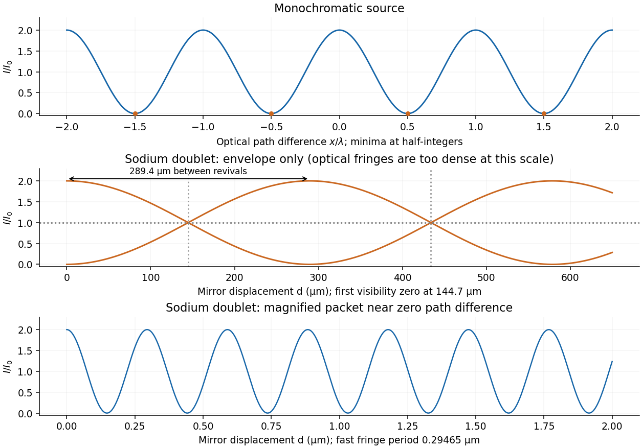
The two sodium lines are distinct optical frequencies, so their rapidly oscillating mutual cross terms average to zero at the detector. Assuming equal line strengths and negligible individual linewidths, add their separate interferograms. Write $\bar{k}=(k_1+k_2)/2$ and $\Delta k=|k_1-k_2|$. With $I_0$ the total mean output intensity,For mirror displacement $d=x/2$ this becomesThis is spectral doublet from Michelson visibility revivals. Since $\Delta \lambda \ll \bar{\lambda }$, $\Delta k\simeq 2\pi \Delta \lambda /{\bar{\lambda }}^2$. Numerically,The first interference visibility zero occurs at $\boxed{d=0.1447\mathrm{mm}}$, with further zeros at odd multiples of that distance. Visibility is restored at integer multiples of $0.2894\mathrm{mm}$. The signed envelope has period $0.5788\mathrm{mm}$: alternate high-visibility packets have opposite fringe phase. Unequal line strengths leave a nonzero minimum visibility, and finite linewidths introduce a further decaying envelope; the wavelength data alone specify neither effect.

Take the two interfering complex amplitudes to have equal intensities $I_0/2$ and relative phase $kx$. The interference cross term then givesThus the mean intensity is $I_0$, the maximum is $2I_0$, and the minima areThe optical path difference period is $\lambda$ and the mirror-displacement period is $\lambda /2$. The assumed equal intensities refer to the two fields at the chosen output, with matching polarization of waves and full optical coherence. They set the normalization; they should not additionally be interpreted as all incident light entering that output port. A physical lossless Michelson interferometer has a complementary second output.

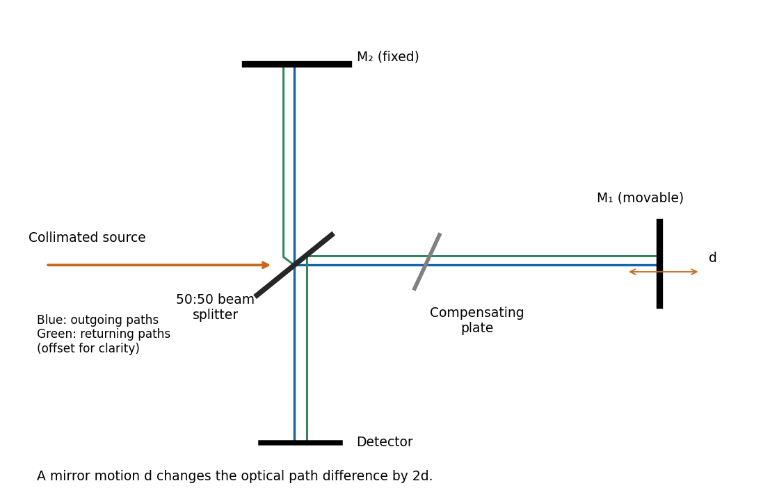
The beam splitter sends transmitted and reflected portions into perpendicular arms. Each mirror returns its beam to the splitter, where the two returning fields recombine towards the detector. A collimating lens provides approximately plane illumination. A compensating plate of the same glass thickness as the beam splitter can equalise the dispersive glass paths, which matters especially for broadband light.

If the arm lengths are ${\ell }_1,{\ell }_2$, the geometric optical path difference in air is $x=2({\ell }_1-{\ell }_2)$, up to a chosen constant and any additional material paths. Moving one mirror by $d$ changes $x$ by $2d$. Fixed reflection phases can be absorbed into the reference position of a bright or dark fringe.

In division of amplitude, one incident beam is split into two or more parts at a partially reflecting interface; they follow distinct paths and are recombined. The Michelson interferometer and thin-film interference use this principle. In division of wavefront, spatially distinct parts of the same wavefront are selected and allowed to overlap, as in double-slit interference. Both require adequate optical coherence; wavefront division particularly exposes the need for spatial optical coherence between the selected regions.

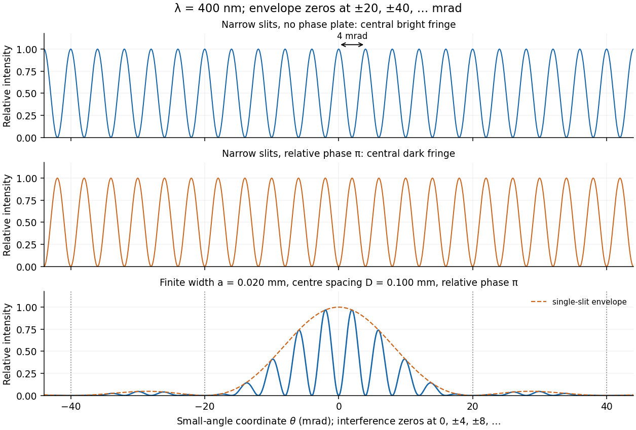
For a rectangular slit centred at $x_c$, the one-dimensional Fraunhofer diffraction integral isThe two equal apertures have centres at $\pm D/2$; the glass subtracts their fields. ThereforeThis is phase-reversed double-slit diffraction: the narrow-slit interference factor is multiplied by the single-slit diffraction envelope. In the limit $a\to 0$, the normalized envelope tends to one, recovering part (d).

The interference minima and envelope minima obey, respectively,Near the axis these are ${\theta }_m\simeq 4m\mathrm{mrad}$ and envelope zeros ${\theta }_n\simeq 20n\mathrm{mrad}$. Here $D/a=5$, so every envelope zero already coincides with an interference minimum. The envelope strongly reduces the outer fringes; its central value is nonzero, but the total intensity still vanishes at $\theta =0$ because the two fields cancel. The sketch uses the small-angle coordinate; the equations above specify the exact angular zeros.

A relative phase $\pi$ changes the sign of one slit field. Their sum becomesThe central interference fringe is now dark. The maxima move to $D\sin \theta =(m+1/2)\lambda$, while the minima occur at $D\sin \theta =m\lambda$. Thus the pattern shifts by half a fringe, $2.00\mathrm{mrad}$ near the axis, but its angular fringe separation remains $\boxed{4.00\mathrm{mrad}}$. This assumes the glass changes phase uniformly and introduces negligible absorption or beam deflection.

Represent equal narrow slits at $x=\pm D/2$ by two contributions with equal complex amplitudes. In a direction $\theta$ the path difference is $D\sin \theta$, soTherefore double-slit interference givesThe bright interference fringes satisfy $D\sin \theta =m\lambda$, with a central maximum. In the small-angle region,Dark fringes lie halfway between bright ones. Exactly, spacing is uniform in $\sin \theta$, not in $\theta$ at large angles. The first panel of the pattern figure below shows the narrow-slit result.

Let the aperture occupy the $z=0$ plane, with coordinates $(x,y)$ and opening $\Sigma$. Write ${\psi }_{\Sigma }(x,y)$ for the incident scalar complex amplitude and $h(x,y)$ for its dimensionless amplitude transmission, including any imposed phase. The observation point has transverse coordinates $(X,Y)$, corresponding to the PDF's $(x_0,y_0)$, and axial distance $R$. Also $k=2\pi /\lambda$ is the wavenumber and $i^2=-1$.

The Huygens-Fresnel principle expresses the propagated field, up to common prefactors and an approximately constant obliquity factor, asIn the paraxial approximation, expand the path asThe last term is negligible in the Fraunhofer diffraction limit, while the first two terms and $1/r\simeq 1/R$ are common across the aperture. Factoring them out leavesIt is the two-dimensional Fourier transform of the transmitted aperture field, evaluated at transverse wavevector $(kX/R,kY/R)$. For appreciable observation angles the corresponding exact directional components are used rather than $X/R,Y/R$.

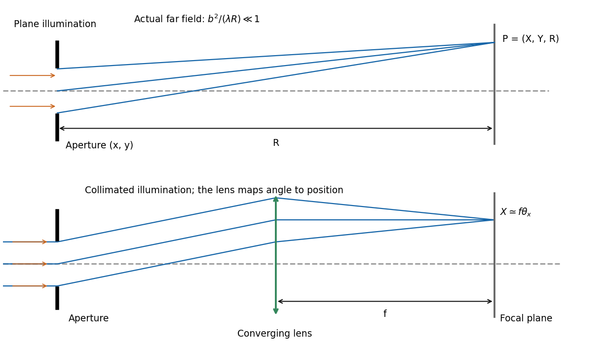
In Fraunhofer diffraction, the relative propagation phase across the aperture is linear in aperture coordinates. If $b$ is its largest transverse size, the neglected quadratic path term must be small: for an observer at distance $R$,For a finite-distance point source a distance $s$ away, also require $b^2/(\lambda s)\ll 1$ if the illumination is to be treated as a plane wave. Numerical factors depend on whether $b$ is a radius or full width and on the permitted phase error; the condition expresses a small Fresnel number.

One can place both source and screen sufficiently far away, or collimate a point source with a lens and observe the aperture in the back focal plane of a second lens. In the latter arrangement rays of each outgoing direction focus at one point, with $X\simeq f{\theta }_x$; the lens removes the need for a physically distant screen. A laser beam approximately uniform across the aperture can supply the incident plane wave. The sketches distinguish an actual far field from its focal-plane equivalent.

The precise bandwidth depends on the output: this is the distinction between displacement and current bandwidths of a series RLC circuit. For current output, or voltage across the resistor, the electrical impedance givesThe half-power points satisfy $|\omega L-1/(\omega C)|=R$. Their positive roots areChanging capacitance shifts the centre without changing this absolute width. For the charge response in part (d), the exact half-height points instead obeywhen both exist their separation only approaches $\gamma =R/L$ at large quality factor. Therefore the printed capacitance-independence claim is exact for current or resistor-voltage output and an approximation for the preceding charge resonance.

For a narrow band-pass filter, use current or resistor-voltage output and make $R/L$ small, counting source, load and inductor losses in the total electrical resistance. Increase $Q=\sqrt{L/C}/R$; if a specified centre frequency is to remain fixed, adjust $C$ with $L$ to keep $LC$ fixed. Capacitor-voltage output alone is not a band-pass response because it has a nonzero DC limit.

The capacitor-charge complex amplitude isFor fixed driving-voltage amplitude, maximizing $|q_0|$ minimizesDifferentiate:The positive-frequency minimum therefore hasThis is the resonance of charge, or capacitor voltage. If the stated inequality fails, their maximum is at zero frequency, and no positive displacement-resonance peak exists. The electric current has the additional factor $\omega$, and instead peaks exactly at ${\omega }_0=1/\sqrt{LC}$ for every $R>0$.

The original diagram is a series RLC circuit, so the same electric current $i=\dot{q}$ passes through all three elements. Choose capacitor electric charge $q$ positive on the plate into which positive $i$ enters. Kirchhoff's voltage law givesDividing by inductance $L$ givesThe correspondence to the forced harmonic oscillator is $m\leftrightarrow L$, $b\leftrightarrow R$, $k\leftrightarrow 1/C$, and $x\leftrightarrow q$. The stored energy is $L{i}^2/2+q^2/(2C)$; its balance is $\dot{E}=Vi-R{i}^2$, confirming the damping sign.

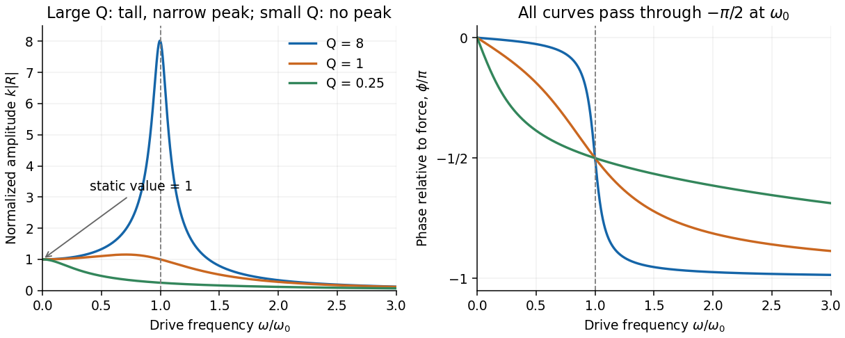
For the steady response of a forced harmonic oscillator, write $x=\mathrm{Re}(A{e}^{i\omega t})$ and use the same complex amplitude convention for the driving force. Substitution givesThus the response magnitude and displacement phase relative to the force areThe phase goes from $0$ at low frequency, through $-\pi /2$ at ${\omega }_0$, towards $-\pi$ at high frequency. The static magnitude is $1/(m{\omega }_0^2)=1/k$, while the high-frequency magnitude is approximately $1/(m{\omega }^2)$.

Define the quality factor by $Q={\omega }_0/\gamma$. If $Q>1/\sqrt{2}$, the displacement peak occurs at ${\omega }_r=\sqrt{{\omega }_0^2-{\gamma }^2/2}$; for $Q\le 1/\sqrt{2}$ the magnitude decreases monotonically from its static value. For $Q\gg 1$ there is a tall narrow peak close to ${\omega }_0$, of height approximately $Q/k$ and width approximately $\gamma$. At very small $Q$ the resonant peak disappears and the response is broad. The plotted functions are normalized as $k|R|$, at fixed $m,k$.

Substituting $x=A{e}^{pt}$ into the damped harmonic oscillator equation givesFor nonnegative viscous damping, the cases areThe PDF's request to express these conditions in terms of $\gamma /m$ is dimensionally inconsistent with its definition $\gamma =b/m$: $\gamma$ already has units ${\mathrm{s}}^{-1}$. With the unnormalised equation $m\ddot{x}+b\dot{x}+kx=0$, the equivalent comparisons are $b/m\gtrless 2{\omega }_0$, or $b^2\gtrless 4mk$. Also ${\omega }_0$ is the undamped natural angular frequency, not in general the driven displacement peak.