A Gaussian distribution with mean $\mu$ and standard deviation $\sigma$ has probability densityIts symmetry, finite variance and simple behavior under linear combinations make it useful for repeated measurements. Roughly $68.3\%$, $95.4\%$ and $99.7\%$ of observations lie within one, two and three true standard deviations of the mean. These are coverage probabilities for a specified distribution, not guarantees that every experimental error is normal.

Why it appears. The central limit theorem explains why many sums of small independent finite-variance contributions approach a Gaussian law after centering and scaling, provided no single contribution dominates. Detector noise, small mechanical disturbances and multiple electronic fluctuations can combine approximately this way. The theorem does not remove a common calibration bias, and it does not justify assuming normal tails for rare large disturbances or arbitrarily correlated errors. A large-mean Poisson distribution also approaches a Gaussian with variance equal to its mean, making normal approximations useful for high-count photon or particle data; low counts require the discrete model.

A classical particle at thermal equilibrium in a one-dimensional harmonic potential has a Gaussian position distribution directly from the Boltzmann distribution:Thus a Gaussian law can arise from the energy dependence of equilibrium probability, rather than only from an informal appeal to many independent errors.

Precision of repeated measurements. For $N$ independent observations with the same mean and variance, the sample mean has variance ${\sigma }^2/N$. For Gaussian observations this mean is exactly Gaussian:Consequently quadrupling the number of independent readings halves the random standard error. When the true variance is unknown, a small-sample confidence interval for a normal mean uses a Student t-distribution with $N-1$ statistical degrees of freedom; replacing that by a normal quantile can overstate precision. Shared systematic errors and correlations do not decrease by the same averaging rule.

Combining results and fitting models. Independent Gaussian estimates $x_i$ of one quantity, with known variances ${\sigma }_i^2$, combine through the inverse-variance weighted meanFor a model $y_i=g_i(\theta )+{ϵ}_i$ with independent zero-mean Gaussian noise, maximizing the likelihood is equivalent to minimizing the weighted least-squares statisticFor a correct linear model with known independent Gaussian errors and $p$ fitted parameters of full rank, the minimized statistic has a chi-squared distribution with $N-p$ degrees of freedom. Nonlinear fits only inherit that familiar approximation under additional regularity and adequate-data assumptions. Known correlated Gaussian errors require the full inverse covariance matrix in the quadratic form.

These properties support confidence intervals, consistency checks, calibration and error propagation. They also give practical diagnostics: inspect residuals for trends, changing spread, correlations or outliers before trusting a Gaussian fit. Gaussian models connect physical fluctuations to quantitative uncertainty, but their assumptions must be checked rather than inferred from the shape of a convenient bell curve.

In this digital-sampling context, Nyquist's theorem means the Nyquist–Shannon sampling theorem. A continuous signal with no Fourier content outside $|f|\le B$ can be reconstructed from uniformly spaced samples taken sufficiently fast. The familiar practical condition isHere $f_N$ is the Nyquist frequency, while $2B$ is the Nyquist rate required by that signal bandwidth. A finite-energy bandlimited formulation allows equality; a rule intended to include arbitrary pure sinusoids at the boundary must be strict, because $\sin (\pi f_{s}t)$ vanishes at every sampling time $t=n/f_s$.

The mechanism is visible in the Fourier transform. Sampling by a time comb creates shifted copies of the original spectrum, separated by $f_s$:If those copies do not overlap, an ideal reconstruction filter selects one copy and recovers the original waveform. Equivalently, ideal interpolation uses the normalized sinc function:Each interpolation function is one at its own sample and zero at all other sample times. Exact reconstruction presumes the bandwidth condition, an ideal sampling clock and the full sample sequence.

If the spectrum extends beyond half the sampling rate, different continuous frequencies become indistinguishable: this is aliasing. A sinusoid at frequency $f$ is indistinguishable on the sampling grid from frequencies differing by integer multiples of $f_s$, with the usual sign reflection for real signals. For example, $10\mathrm{kHz}$ sampled at $8\mathrm{kS}{\mathrm{s}}^{-1}$ aliases to $2\mathrm{kHz}$; a later digital filter cannot tell which signal generated those samples.

Use an analogue anti-aliasing filter before the analogue-to-digital converter and choose a sampling rate leaving room for its finite transition band. Faster sampling can relax that analogue filtering problem, but simply increasing the number of samples in a fixed-duration record does not improve the independent Fourier-bin spacing beyond approximately $1/T$. A long recording is needed for low-frequency resolution, while a small sampling interval is needed for high-frequency coverage. Finite records also introduce windowing and spectral leakage.

Digitization adds amplitude quantization as well as time sampling. An ideal $N$-bit converter spanning voltage range $V_{\mathrm{span}}$ has step $\Delta =V_{\mathrm{span}}/2^N$. When quantization error may be modeled as independent and uniform across one step, its rms size is $\Delta /\sqrt{12}$; small coherent signals need not obey that white-noise approximation. Sampling rate controls temporal ambiguity, recording duration controls frequency resolution, and converter resolution controls amplitude discretization.

Electrical noise reduction starts by identifying what is unwanted in the measured signal and where it enters. Increasing gain amplifies both signal and input noise; it does not by itself improve the input signal-to-noise ratio. Separate intrinsic component fluctuations, amplifier noise and external pickup before choosing a remedy.

Physical sources. A resistor at temperature $T$ has classical one-sided open-circuit thermal electrical noise density $S_V=4k_{B}TR$ per hertz. In a flat measurement bandwidth $B$, its rms voltage is $\sqrt{4k_{B}TRB}$. Lowering an appropriate resistance, reducing temperature or narrowing the useful bandwidth can reduce this noise, with loading and signal-gain tradeoffs considered. These are power spectral densities; an amplitude spectral density is their square root.

Discrete independent charge transfers give shot noise, with one-sided current density $S_I=2eI$ in the simple Poisson process model. Reducing leakage or unwanted bias current can help, but reducing a photocurrent may also reduce the desired signal. Charge correlations can change the simple shot-noise law. At low frequency, flicker noise and drift often dominate and are not described by a white spectrum.

Amplifier and impedance choice. An operational amplifier has equivalent input voltage and current noise. In a simplified uncorrelated model, a resistive source contributes the input-referred voltage densityHere $e_n,i_n$ are the voltage and current amplitude spectral densities and $Z_s$ is the source electrical impedance; feedback components add further terms in a full circuit. Low current noise matters particularly for a high-impedance source, while voltage noise can dominate for a low-impedance source. Minimize needless source impedance, leakage and long sensitive connections without sacrificing the required transduction gain or bandwidth. Bias-current offsets and thermal drift also require calibration; they are not removed simply by quoting a random-noise density.

Pickup and bandwidth. Shield sensitive circuits against electric-field coupling, minimize loop area to reduce changing magnetic-flux pickup, and use twisted signal/return pairs or suitable coaxial connections. Differential readout rejects common-mode interference when impedances and amplifier responses are adequately matched. Plan the signal returns to avoid unwanted circulating ground currents, and decouple supply rails locally so supply fluctuations do not enter the signal path. Mechanical vibration, cable motion and temperature changes may be converted into electrical noise as well.

A low-pass filter removes out-of-band noise before digitization; an anti-aliasing filter is needed because digital filtering cannot undo already aliased content. Avoid a narrower passband than the physical signal requires. For a known periodic signal, modulation and a lock-in amplifier select a narrow frequency interval, often moving the measurement above a strong flicker noise region. A notch can reject a narrow interference line if that does not remove essential signal information.

Independent noise contributions add in variance, not directly in rms amplitude. Averaging $N$ independent equal-variance readings reduces the standard error by $N^{-1/2}$, but slow correlated drift and systematic errors need separate controls. Good noise reduction preserves the information-bearing signal while reducing unwanted coupling, intrinsic fluctuations or the admitted noise bandwidth.

A Hermitian operator satisfies the adjoint symmetry conditionfor vectors in its specified domain. For a finite matrix this means $A=A^{†}$. For an unbounded differential operator, boundary conditions and domains matter: symmetry on a chosen domain is not alone sufficient for self-adjointness. Physical observables require the corresponding self-adjoint operator and its spectral measure. This distinction prevents purely formal integration by parts from being mistaken for a complete operator definition.

Real eigenvalues. If $A|a⟩=a|a⟩$ with nonzero norm, Hermiticity impliesso $a=a^{\ast }$. Thus eigenvalues representing measurement outcomes are real.

Orthogonality. For eigenvectors $|a⟩,|b⟩$,Hence $(a-b)⟨b|a⟩=0$, and distinct eigenvalues have orthogonal eigenvectors. Within a degenerate eigenspace, Gram-Schmidt orthogonalization can choose an orthonormal basis. In finite dimensions the spectral theorem gives a complete orthonormal eigenbasis andwhere $P_a$ projects onto each eigenspace. In infinite dimensions a continuous spectrum may require a spectral integral rather than a normalizable eigenvector for every possible outcome; a position operator on the full line is a familiar example.

Measurements and probabilities. In the discrete case the Born rule assigns probability $⟨\psi |P_a|\psi ⟩$ to the outcome $a$. For a nondegenerate eigenbasis, $|\psi ⟩={\sum }_a{c}_a|a⟩$ gives probabilities $|c_a{|}^2$, withThe variance vanishes precisely when the state lies in an eigenspace with a single sharp outcome. A repeatable ideal projective measurement prepares the corresponding eigenspace; superpositions of different eigenvalues do not have a preassigned sharp value of that observable in this description.

Compatibility and dynamics. Commuting Hermitian matrices admit simultaneous diagonalization, permitting a common set of sharp labels. For example $L^2,L_z$ commute, whereas $L_x,L_y$ do not. In the differential-operator setting the corresponding spectral compatibility requires appropriate domain conditions. Noncommuting observables obey the Robertson uncertainty principleThe canonical commutation relation then gives $\Delta x\Delta p\ge \hslash /2$.

The Hamiltonian operator represents energy. A self-adjoint $H$ generates unitary time evolution, $U(t)=e^{-iHt/\hslash }$, preserving norm and total probability; its eigenvalues determine stationary-state phases and transition energies. Hermiticity supplies real outcomes and orthogonal eigenspaces, while self-adjointness and the spectral theorem make these measurement and evolution rules mathematically complete.

Ehrenfest theorem relates the dynamics of quantum expectation values to operator commutators. For a normalized state obeying $i\hslash |\dot{\psi }⟩=\hat{H}|\psi ⟩$ and a possibly time-dependent observable $\hat{A}$, differentiate $⟨A⟩=⟨\psi |\hat{A}|\psi ⟩$. Using the adjoint Schrödinger equation for the bra givesThusThe identity assumes a common domain on which the required products and derivatives are defined.

For $H=p^2/(2m)+V(x)$, the canonical commutation relation gives $[x,H]=i\hslash p/m$ and $[p,H]=-i\hslash V^{\prime }(x)$. ThereforeThese resemble Hamilton's equations and Newton's second law, but generally $⟨V^{\prime }(x)⟩\ne V^{\prime }(⟨x⟩)$. If the state is localized about $\overline{x}=⟨x⟩$, a local expansion givesThe classical trajectory equation for the mean is accurate when the force changes little across the wave packet. For a quadratic harmonic potential, $V^{\prime }$ is linear and this closure is exact for every state with the relevant finite moments: $m{d}^2⟨x⟩/d{t}^2=-m{\omega }^2⟨x⟩$. This exact classical evolution of the centroid does not eliminate its quantum position uncertainty or make every state a point particle.

The correspondence principle is broader: quantum predictions recover classical ones in an appropriate limit, such as large action compared with $\hslash$ and observations that cannot resolve individual quantum levels. It is not the assertion that every large quantum number automatically makes every possible state classical. Delocalized superpositions and interference can remain significant unless the physical preparation and measurement justify a classical description.

A spectral example is useful. For a quantum harmonic oscillator, neighboring levels differ by $\hslash \omega$, giving transition frequency $\omega /(2\pi )$, equal to its classical oscillation frequency. A coherent state makes the connection more concrete: its mean position and momentum oscillate classically while the finite-width Gaussian profile retains its quantum uncertainty. For hydrogenic Bohr levels $E_n=-A/n^2$, transitions between nearby large $n$ have $\Delta E/\hslash \simeq 2A/(\hslash n^3)$, which equals the classical circular orbital angular frequency in that model. Ehrenfest's theorem supplies an exact expectation-value bridge; a classical trajectory follows only when the force can also be evaluated at the mean position.

The Bohr model combines classical circular motion in the Coulomb potential with explicitly quantum postulates. A one-electron atom of nuclear charge $+Ze$ has electron–nucleus reduced mass $\mu$. With $C=Z{e}^2/(4\pi {\epsilon }_0)$, the relative circular orbit obeysBohr postulates permitted nonradiating stationary orbits with $L=n\hslash$, for $n=1,2,\dots$. These assumptions giveFor hydrogen with the nucleus taken infinitely heavy, the $n=1$ radius is the Bohr radius, $a_0\simeq 5.29\times 10^{-11}\mathrm{m}$. The finite reduced mass gives the small nuclear-motion correction, and increasing $Z$ contracts the one-electron orbit.

The circular-motion equation gives $T=C/(2r)$ while the potential energy is $-C/r$, so the total energy is $-C/(2r)$. Substituting the quantized radius yieldsFor the heavy-nucleus hydrogen approximation, $E_n\simeq -13.6\mathrm{eV}/n^2$. The ionization threshold is zero energy, so removing the ground-state electron requires about $13.6\mathrm{eV}$.

The model further postulates that radiation is emitted or absorbed only in transitions between stationary orbits, with photon energy $h\nu =|E_i-E_f|$. Emission from $n_i>n_f$ givesThus it reproduces the principal hydrogen spectral series, their limiting wavelengths, and the gross hydrogenic energy levels. For example, $n=3\to 2$ in hydrogen has $\Delta E\simeq 1.89\mathrm{eV}$ and $\lambda \simeq 656\mathrm{nm}$, a visible line. Absorption reverses the transition when the photon matches the energy gap.

The achievement is that quantized energies explain discrete spectra, but the model's stationary orbits are postulates rather than consequences of classical electrodynamics: an accelerating classical charge would radiate. It does not provide a general calculation of line intensities or transition selection rules and fails as a quantitative theory of many-electron atoms. Spin, fine structure and the full Zeeman effect require further physics. Modern quantum mechanics replaces definite electron orbits by wavefunctions and quantum probabilities. In particular, the true hydrogen ground state has $\ell =0$, so its orbital angular momentum vanishes; the model's rule $L=n\hslash$ should not be identified with the modern orbital eigenvalue rule $L^2=\ell (\ell +1){\hslash }^2$. Bohr's energy quantization remains a successful hydrogenic approximation, while its literal orbital picture does not.

Using the observed counts,ThusTogether with the $67\%$ direct ground state branch, these sum to unity. No measurement uncertainties were supplied for these ratios, so the extra digits only document the arithmetic.

Let $K$ be the common normalization converting the quoted $N_i$ to photon numbers per parent decay. Apply nuclear level population balance to scheme A, starting with the top level:For example, the $3\to 2$ transition contributes $K{N}_2$ to the population of level 2; it must be subtracted from the total leaving level 2 to obtain its direct beta feeding. Similarly, a photon in the strong $1\to 0$ line need not imply a direct beta transition to level 1.

The three equations giveAdding them cancels the internal cascade counts:This also has a simple physical meaning: each decay that initially feeds an excited daughter eventually contributes exactly one of the three transitions into the ground state. The number of all emitted photons is not the correct normalization, because a single cascade can emit several.

Consequently the required formulae are

The four direct beta decay branching fractions exhaust the parent decays in the model, soHere the question's ${\Gamma }_i$ are dimensionless branching fractions, despite the conventional use of $\Gamma$ for a dimensionful decay width. Its “zeroth excited state” means the daughter ground state. Cascades through an excited level do not count as an additional direct beta branch to it.

Retain $a_y,a_z,b_y,b_z$ as defined in Case 1. In the laboratory, A moves and B is stationary. Transform A's fields and add B's unchanged electrostatic field:The laboratory linear charge densities are ${\lambda }_A=\gamma \eta$ and ${\lambda }_B=\eta$, with electric currents $I_A=\gamma \eta v$ and $I_B=0$.

In $O^{\prime }$, A is stationary while B moves with velocity $-v\hat{\mathbf{x}}$. Thus A contributes its rest electrostatic field, and B contributes the boosted electric field and the opposite-sign convective magnetic field:The densities in this frame are ${\lambda }_A^{\prime }=\eta$, ${\lambda }_B^{\prime }=\gamma \eta$, with $I_A^{\prime }=0$ and $I_B^{\prime }=-\gamma \eta v$. Substituting the laboratory result into part (a) gives the same fields; for instance $E_y^{\prime }=\gamma [(\gamma a_y+b_y)-v\gamma v{a}_y/c^2]=a_y+\gamma b_y$. The magnetic contribution attributed to A disappears in its own frame, but B's contribution does not.

Write $a_y=E_{A,y}^0$, $a_z=E_{A,z}^0$, $b_y=E_{B,y}^0$ and $b_z=E_{B,z}^0$, evaluated at the same transverse coordinates $(y,z)$. A superscript $0$ labels each filament's own rest frame, rather than a single common frame in all cases. The filaments are infinite and uniform along $x$, so the change of longitudinal coordinate under a Lorentz boost creates no extra dependence in these functions. After the acceleration transients have passed, the magnetic field of each filament vanishes in its own rest frame.

For a filament moving at $+v\hat{\mathbf{x}}$, use the inverse of part (a): its transverse electric field in the laboratory is $\gamma {\mathbf{E}}^0$ and its magnetic field is $\mathbf{v}\times \mathbf{E}/c^2$. Superposition for the two co-moving filaments therefore gives, in $O$,In the common co-moving frame $O^{\prime }$ both filaments are at rest, soFor example, $B_y^{\prime }=\gamma [-\gamma v(a_z+b_z)/c^2+v\gamma (a_z+b_z)/c^2]=0$, a useful sign check. The supplied $\eta$ is the proper linear charge density. Thus each laboratory density is $\gamma \eta$ and each laboratory electric current is $\gamma \eta v$, consistently with length contraction and the four-current transformation. In $O^{\prime }$ each density is $\eta$ and both currents vanish.

Keep source, observer and magnetic field in their original places, but interchange the physical polarizers, including their pass-axis orientations. The forward order is then $P_2$, glass, $P_1$, so the new Jones matrix is again $P_{1}R(\theta )P_2$. ConsequentlyThis is the same intensity change as exchanging source and observer. At the field that maximizes the original forward transmission, the swapped arrangement blocks the beam. If both operations were performed together, the original order relative to propagation would be restored and so would the original transmission. The answer concerns exchanging the two differently oriented pass axes; simply relabelling two identical polarizers while leaving their axes fixed would not change the apparatus.

Keep the magnetic field fixed in the laboratory and exchange source and observer. The incident unpolarized light now meets $P_2$ first. In fixed transverse laboratory axes the backward glass map is still $R(\theta )$, not $R(-\theta )$: this is optical nonreciprocity of the Faraday effect. The order of the two polarizers is reversed, soThe reverse light intensity is thereforeFor the optimal forward setting $\theta =\pi /4$, it vanishes: the $45^{\circ }$ input selected by $P_2$ rotates to $90^{\circ }$ and is blocked by $P_1$. At a general field, $I_r+I_f=I_0/2$. The result assumes equal incident light intensities in the two experiments. Treating the glass as a reciprocal natural optical rotator would predict cancellation of its laboratory rotation on reversal and would give the wrong answer here.

The lower derivative index and the upper electromagnetic four-potential index are fully contracted. For a constant Lorentz transformation,HenceThis is a statement about Lorentz transformations, not electromagnetic gauge transformations. The quantity is not generally gauge invariant; setting it to zero is the Lorenz gauge condition, which is Lorentz covariant because zero remains zero in every inertial frame.

The chain rule givesThusDifferentiation with respect to a contravariant coordinate has a lower transformation index. In inertial Cartesian coordinates in Minkowski spacetime, no connection term is needed for this coordinate transformation of a derivative acting on a scalar; Lorentz transformations have constant Jacobians.

First lower the index of the four-current with the Minkowski metric: $J_{\beta }=g_{\beta \alpha }{J}^{\alpha }$. The displayed expression is thenThereforeIts one free lower index transforms with the inverse coordinate Jacobian. The contraction with the metric here lowers an index; it does not make the current a scalar because the index $\delta$ remains free.

The upper index identifies $P^{\alpha }$ as a contravariant Lorentz four-vector, obeying the rank-one contravariant tensor transformation law. Its components transform with the coordinate Jacobian,It is not invariant component by component. Its contracted square $P_{\alpha }{P}^{\alpha }=m^2{c}^2$, for metric signature $(+,-,-,-)$, is a Lorentz invariant. This distinguishes a contravariant transformation law from an invariant scalar.

Let each drive region have length $\ell$ and the drive-free gap have length $L$, measured edge to edge. A particle of constant speed $v>0$ experiences $\tau (v)=\ell /v$ and $T(v)=L/v$. For a normalized detected-beam speed probability density function $f(v)$, sum the transition probabilities, not the probability amplitudes of different particles:The displayed $f$ is an ideal effusion flux distribution, with speed scale $u$, uniform transmission and speed-independent detection efficiency. It is not a claim about any particular clock's selected beam. The substitution $x=(v/u{)}^2$ gives $f(v)dv=x{e}^{-x}dx$, proving normalization. Actual apertures, state selection and readout can change the effective weights.

For an original example choose $\ell =0.10\mathrm{m}$, $L=1.00\mathrm{m}$, $u=v_{\ast }=200\mathrm{m}{\mathrm{s}}^{-1}$ and $\Omega =2\pi \times 500\mathrm{rad}{\mathrm{s}}^{-1}$. The reference particle has ${\tau }_{\ast }=0.500\mathrm{ms}$, $T_{\ast }=5.00\mathrm{ms}$ and resonant $\pi /2$ pulses. The instantaneous-pulse width would be $100\mathrm{Hz}$. The exact finite-pulse width for that single speed is about $88.7\mathrm{Hz}$; the chosen distribution also reduces the on-resonance average to approximately $0.738$ because not every particle receives a $\pi /2$ pulse.

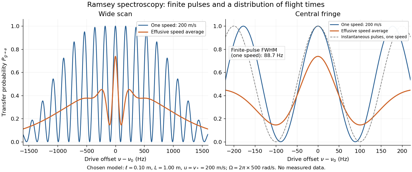
Different velocities smear side fringes because $\delta L/v$ varies across the beam. Nevertheless every term is even in $\delta$, so this symmetric ideal-model average has no odd line asymmetry that could displace the central lock point. Reduced contrast or altered width alone is not evidence of a shifted line center. A speed-dependent transition shift or unequal drive quantum phases changes that conclusion; atomic clock frequency shifts explains why these distinctions matter experimentally.

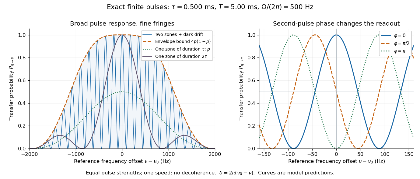
Keep the first pulse's oscillation phase zero and give the second phase $\phi$ in the Driven two-level Rabi model. Its upper off-diagonal Hamiltonian operator entry is $\hslash \Omega e^{-i\phi }/2$. Multiplying the two pulse unitary operators and the free-flight unitary operator givesThe Born rule gives the displayed phase-dependent form using the $p,b,\theta$ of the Ramsey fringe envelope. Thus $\phi =0$ reproduces the existing expression, while $\phi =\pi$ turns a resonant transfer maximum into zero transfer. A single pulse's population is insensitive to its drive phase; the second coherent interaction makes their difference observable. An uncontrolled, uniformly random $\phi$ instead averages this probability to $2p(1-p)$, leaving the broad pulse response but removing the dark-flight fringes.

Finite pulses also contribute to the near-resonant frequency slope. For $\Omega \tau =\pi /2$, differentiating $\theta$ at $\delta =0$ gives ${\theta }^{\prime }(0)=1/\Omega$. Consequently the phase near resonance isAt $\phi =\pi /2$ the exact resonant slope is $\partial P/\partial \nu =-\pi T_{\mathrm{eff}}$. For the plotted parameters $T_{\mathrm{eff}}\simeq 5.637\mathrm{ms}$; the near-resonant estimate $1/(2T_{\mathrm{eff}})\simeq 88.71\mathrm{Hz}$ explains why the exact finite-pulse width below differs from $100\mathrm{Hz}$. The slope is exact at resonance under these assumptions, while this width estimate uses the local phase expansion. A velocity distribution requires averaging the full response, not substituting one effective flight time.

The exact finite-pulse Ramsey transition probability separates a slowly varying pulse response from rapid quantum interference. Define the single-zone transfer probability $p$ and a pulse-induced quantum phase $\theta$ bySince $c_p^2+b^2=1-p$, factorizing the real bracket in the original formula givesWhere $c_p=b=0$, the probability is zero and $\theta$ need not be defined. Elsewhere this identity proves the envelope bound without a weak-drive assumption. The envelope $4p(1-p)$ is not the single-zone response $p$: two equal coherent interactions have different transfer weights. A contiguous resonant Rabi pi pulse of duration $2\tau$ provides another useful comparison with the same total drive duration, but no dark interval. Its line is broad because it has no long flight phase.