For small oscillations with quadratic kinetic and potential energies, a normal mode has a fixed spatial amplitude pattern and one angular normal frequency. Its amplitude is a normal coordinate; choosing all modes diagonalizes the two quadratic forms and decouples their equations. A zero frequency describes a free symmetry motion.

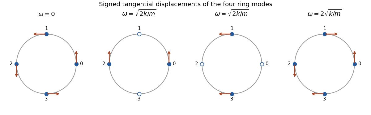
Let $q_j=R[{\theta }_j-j\pi /2]$ be the small signed arc displacements, with cyclic indices $j=0,1,2,3$. The springs follow arcs, so their extensions are $q_{j+1}-q_j$. The Lagrangian of the normal modes of a four-bead spring ring isThe stiffness matrix divided by $k$ is the cycle graph Laplacian, with diagonal entries two, adjacent entries minus one, and zero opposite entries. An orthonormal basis of mode vectors and their frequencies isThe normal mode coordinates are $Q_{\alpha }=u_{\alpha }\cdot q$, with equations ${\ddot{Q}}_{\alpha }+{\omega }_{\alpha }^2{Q}_{\alpha }=0$. The zero mode rotates all beads together without stretching a spring and has $Q_0=A+Bt$. In each of the two degenerate middle modes, opposite beads have opposite signed arc displacements while the other pair remains stationary. Any fixed linear combination is another mode of that frequency. The last mode alternates the signed displacement of adjacent beads. The radius cancels from the frequencies because arc length supplies the same factor $R^2$ to the angular kinetic and spring energies.

The one-sided Laplace transform is $\bar{f}(p)={\int }_0^{\infty }{e}^{-pt}f(t)dt$. Its Bromwich inversion formula is $f(t)=(2\pi i{)}^{-1}{\int }_{\gamma -i\infty }^{\gamma +i\infty }{e}^{pt}\bar{f}(p)dp$, with an upward vertical contour to the right of all singularities and within the appropriate convergence half-plane.

To derive the convolution theorem for Laplace transforms, transform $x(t)={\int }_0^{t}f(\tau )g(t-\tau )d\tau$. With $u=t-\tau \ge 0$, the triangular integration region becomes a quadrant. Fubini's theorem gives $\bar{x}(p)={\int }_0^{\infty }{\int }_0^{\infty }{e}^{-p(u+\tau )}f(\tau )g(u)dud\tau =\bar{f}(p)\bar{g}(p)$, under the usual absolute convergence hypotheses. Inversion gives the required convolution formula.

For the differential equation, the transformed initial conditions give $(p^2-1)\bar{y}=\bar{g}+p+1$, hence $\bar{y}=\bar{g}/(p^2-1)+1/(p-1)$. Since $\mathcal{L}[\sinh t]=1/(p^2-1)$ for $\mathrm{Re}p>1$, the convolution yieldsThe integral and its first derivative vanish at zero, so the homogeneous term supplies both initial values. Differentiating twice gives the forcing through the unit derivative of the hyperbolic-sine kernel at zero.

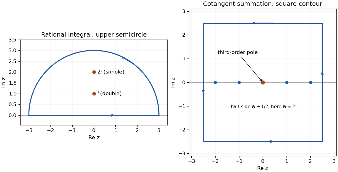
For a pole of order $N$ at $z_0$, the residue is ${\mathrm{Res}}_{z_0}F=\frac{1}{(N-1)!}{\lim }_{z\to z_0}\frac{d^{N-1}}{d{z}^{N-1}}[(z-z_0{)}^{N}F(z)]$. For the rational integral, close the real-axis contour with an upper semicircle. The poles are double at $i$ and simple at $2i$, withThe arc integral vanishes as $O(R^{-5})$. By the residue theorem the whole real-axis integral is $\pi /9$, and evenness givesFor the second calculation, reciprocal expansion of the sine gives $1/\sin z=z^{-1}+z/6+O(z^3)$. Multiplying by $\cos z=1-z^2/2+O(z^4)$ yields $\cot z=z^{-1}-z/3+O(z^3)$. ThereforeAt every nonzero integer $n$, $\pi \cot \pi z$ has a simple pole with residue one, giving residue $1/n^2$ after division by $z^2$.

The cotangent contour summation uses the positively oriented square of half-side $R=N+1/2$. Its length is $8R$ and $|z|\ge R$ on its boundary. The supplied cotangent bound implies $|\oint Fdz|\le 8\pi C/R\to 0$. Its enclosed residues sum to $-{\pi }^2/3+2{\sum }_{n=1}^N{n}^{-2}$. The residue theorem therefore proves the Basel problem value

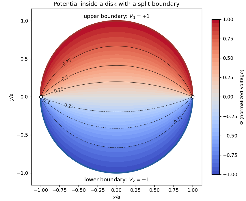
For Laplace's equation in polar coordinates, put $\Phi =R(r)\Theta (\theta )$. Separation of variables gives ${\Theta }^{\prime \prime }+n^2\Theta =0$ and $r^2{R}^{\prime \prime }+r{R}^{\prime }-n^{2}R=0$. Periodicity selects integers $n\ge 0$. For $n>0$, the radial solutions are $r^n,r^{-n}$; for $n=0$, they are $1,\ln r$, while a term linear in $\theta$ is excluded by periodicity. Their superposition isInside the disk, boundedness at the origin removes the logarithm and all negative powers. The separately biased semicircular boundary values have mean $(V_1+V_2)/2$, no nonconstant cosine coefficients, and sine coefficients $2(V_1-V_2)/(\pi n)$ for odd $n$, zero for even $n$. The disk potential with two semicircular boundary values is thereforePut $w=(r/a)e^{i\theta }$. The odd logarithmic series sums to ${\sum }_{m\ge 0}{w}^{2m+1}/(2m+1)=\frac{1}{2}\log [(1+w)/(1-w)]$. The quotient has positive real part for $|w|<1$, so its argument is the principal arctangent of $2(r/a)\sin \theta /[1-(r/a{)}^2]$. Taking imaginary parts givesThe boundary limits away from the two voltage jumps are $V_1,V_2$. Along the diameter through a jump the value is the mean; incompatible adjacent boundary limits prevent a continuous extension at the junctions.

An invariant subspace $W$ satisfies $D(g)W\subseteq W$ for every $g\in G$; applying the inverse gives equality. The representation is irreducible when the only invariant subspaces are $0$ and the full space.

The inverse and conjugate transpose each reverse multiplication order, so their combination preserves it:Its values are invertible, so this is the conjugate contragredient representation.

If $W$ is invariant under $D_2$, take $w\in W$ and $v\in W^{\perp }$. For the standard Hermitian inner product,since $D_2(g^{-1})w\in W$. Hence $D_1(g)v\in W^{\perp }$, proving its invariance. If $D_1$ is irreducible, $W^{\perp }$ is either zero or the whole space; finite-dimensional orthogonal complementation makes $W$ the whole space or zero, respectively. Thus $D_2$ is irreducible whenever $D_1$ is irreducible.

Choose the Green function convention ${\Delta }_{\mathbf{r}}G(\mathbf{r};{\mathbf{r}}_0)={\delta }^{(3)}(\mathbf{r}-{\mathbf{r}}_0)$, with decay at infinity and no extra singularities. For sufficiently decaying source data,Away from its source, this fundamental solution of the Laplace equation is harmonic. Its radial derivative is $1/(4\pi {\rho }^2)$, so the flux of its gradient through a small source-centred sphere is one. The divergence theorem therefore supplies exactly the unit Dirac delta function required by the equation. Decay at infinity excludes an added globally regular harmonic term.

For the half-space, reflect the source to ${\mathbf{r}}_0^{\ast }=(-x_0,y_0,z_0)$. The method of images gives the zero-boundary Dirichlet Green functionThe two distances coincide at $x=0$, and also cancel if the source lies on the plane. The image singularity lies outside the physical domain.

The sign conventions for a Dirichlet Green function require care here. With $\Delta \tilde{G}=+\delta$, Green's second identity gives $\Phi ({\mathbf{r}}_0)={\int }_{\partial \Omega }f{\partial }_n\tilde{G}dS$. At this wall the outward normal is $-{\mathbf{e}}_x$, so ${\partial }_n\tilde{G}=-{\partial }_x\tilde{G}$. Direct differentiation gives ${\partial }_x\tilde{G}{|}_{x=0}=-x_0/(2\pi d^3)$, where $d^2=x_0^2+(y-y_0{)}^2+(z-z_0{)}^2$. Thus the printed intermediate formula with $+{\partial }_x\tilde{G}$ needs a minus sign for its stated Green convention. The final Poisson kernel for the upper half-space is positive:Its boundary integral is one for constant data, providing an independent sign check.

Apply the Euler-Lagrange equation to the integrand of $F-\lambda G$, namely $p{y}^{\prime 2}-q{y}^2-\lambda r{y}^2$. With fixed zero endpoint values, it gives $(p{y}^{\prime }{)}^{\prime }+qy+\lambda ry=0$. Multiplying by $y$ and using integration by parts gives $F=\lambda G$, so each stationary Rayleigh quotient $F/G$ equals its eigenvalue.

In the half-line problem, $p=x$, $q=-x$, $r=1$, so the quotient is $R[y]={\int }_0^{\infty }x(y^{\prime 2}+y^2)dx/{\int }_0^{\infty }{y}^{2}dx$. For $y=e^{-\beta x}$, $\beta >0$, its numerator is $({\beta }^2+1)/(4{\beta }^2)$ and denominator $1/(2\beta )$. Hence $R=(\beta +{\beta }^{-1})/2$, minimized at $\beta =1$:For the compactly supported linear trial, $A>0$, the numerator is $A^2/2+A^4/12$ and denominator $A^3/3$. Thus $R=3/(2A)+A/4$, minimized at $A=\sqrt{6}$, givingThe derivative jump at the cutoff is allowed in the quadratic-form trial space of the Rayleigh-Ritz method: the trial is continuous and has finite form energy.

The exponential ground state of a linearly weighted Sturm-Liouville problem proves which estimate is best. Vanishing endpoint terms giveEquality occurs for $y=C{e}^{-x}$, which also satisfies the differential equation with $\lambda =1$. Thus the exponential trial gives the exact smallest eigenvalue, whereas the linear trial gives a larger upper bound. Finiteness at the singular endpoint supplies the regular branch with $xy{y}^{\prime }\to 0$; all the displayed trials have the required vanishing boundary terms.

For the zero initial data, the Green function of an undamped oscillator is $G_0(x,s)=\sin [k(x-s)]/k$ for $0\le s\le x$, and zero for $s>x$. It is continuous at the source and its first derivative jumps by one. The resulting convolution isIt vanishes together with its first derivative at zero and has the required resonant forcing.

For the two-endpoint problem, write $L=\pi /(6k)$, $a=\min (0,L)$, $b=\max (0,L)$ and $\kappa =|k|$. This covers both signs of the supplied nonzero $k$. Left and right homogeneous solutions are $\sin [\kappa (x-a)]$ and $\sin [\kappa (b-x)]$, with Wronskian $-\kappa \sin [\kappa (b-a)]$. The Dirichlet Green function is thereforeIts endpoint values are zero and its first derivative jumps by one. Here $\kappa (b-a)=\pi /6$, so the denominator does not vanish. Integrating the constant forcing givesEquivalently $y=(1-\cos kx)/2+(\sqrt{3}/2-1)\sin kx$. The negative interior response is consistent with the negative kernel for this short Dirichlet interval.

Multiply the original equation by $p(x)=\exp ({\int }^{x}u(s)ds)>0$. Since $p^{\prime }=up$, it becomes $(p{y}^{\prime }{)}^{\prime }+qy+\lambda ry=0$ with $q=pv$, $r=pw>0$. This is Sturm-Liouville form. For two real eigenfunctions, multiply the equation for $y_n$ by $y_m$, subtract the equation for $y_m$ multiplied by $y_n$, and integrate. The Lagrange identity for a Sturm-Liouville operator givesEach separated homogeneous boundary condition makes the corresponding determinant zero, provided its pair of coefficients is not both zero. For distinct eigenvalues, this proves the orthogonality of Sturm-Liouville eigenfunctions.

For the constant drift, the drift-removing substitution for a Dirichlet Sturm-Liouville problem is $y=e^{-\alpha x}v$. It reduces the equation to $v^{\prime \prime }+\lambda v=0$ with $v(0)=v(\pi )=0$. Nonzero solutions occur exactly atThe zero and negative values give only the zero solution under both endpoint conditions. The self-adjoint expression is $(e^{2\alpha x}{y}^{\prime }{)}^{\prime }+{\alpha }^2{e}^{2\alpha x}y+\lambda e^{2\alpha x}y=0$. Hence the weight is $r=e^{2\alpha x}$, and for the displayed normalization,

A matrix is diagonalizable if some invertible $S$ makes $S^{-1}AS$ diagonal, equivalently if it has a basis of eigenvectors. If $A^p=0$ and $Av=\lambda v$ for $v\ne 0$, then $0=A^{p}v={\lambda }^{p}v$, so every eigenvalue is zero. There is at least one zero eigenvalue: otherwise $A$ and hence $A^p$ would be invertible. A diagonalizable nilpotent matrix has an all-zero diagonal form and therefore is zero itself.

For the specified matrices, direct determinant expansion givesThe Cayley-Hamilton theorem gives $B^3=0$. Its entry $B_{12}=-2$ is nonzero for every real $\alpha$, so $B$ is not diagonalizable for any $\alpha$. The matrix $C$ has three distinct real eigenvalues and is therefore diagonalizable over $\mathbb{R}$. For an explicit check, take columns $(-1,0,1{)}^T$, $(2,-3,1{)}^T$, $(2,3,1{)}^T$ in $S$; then $S^{-1}CS=\mathrm{diag}(-6,0,6)$.