Topics (384k) Articles (398k) Users (410) Discussions (242) Comments (383) Files (13k) New article

Let be the number of projectiles actually incident on the foil during an exposure, its foil areal number density, and the probability of detecting an accepted particle. For a sufficiently small detector patch of area at distance from the scattering point, with its normal at angle to the line of sight,The product is a dimensionless scattering probability in this approximation; is an expected value of counts, so it need not be an integer. The approximation requires a nearly constant differential scattering cross-section and efficiency across the patch and incident beam. For finite acceptance use , including the incident beam's spread if appreciable. A screen facing the foil has .
For an original numerical model, stipulate monoenergetic alpha particles with , , and a gold target with . Use the rounded model constant , where electronvolts and . Thus and . Choose , , , and . For example, facing the foil at gives this small-patch solid angle.
At , and , using barn . The expected signal is counts. At it is four times larger, about counts. Doubling foil areal number density or detector solid angle doubles these expected signals as long as the approximations continue to hold.
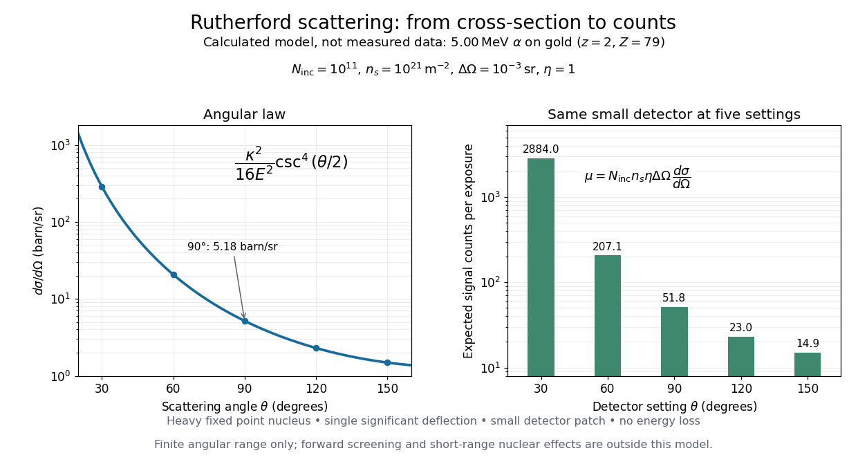
Calculated Rutherford angular cross-section and finite-detector counts
. Original calculation for the stated ideal monoenergetic alpha beam and thin gold foil. The curve is a differential cross-section; the bars are expected counts for the specified small detector solid angle at separate settings. They are not measured 1909 or 1913 data, and do not sum to a total scattering probability. The curve is shown only from 20 to 160 degrees. Details.An observation also contains backgrounds. For a stable source and matched geometry, an estimator is , where denotes exposure duration. If source activity changes, normalize by incident exposure as well. Background subtraction removes an estimated background; it does not make finite counting fluctuations disappear.
For an incident beam uniform across its relevant impact parameters, an incident annulus has area . Rotational symmetry maps it to outgoing solid angle . The central-potential classical differential cross-section and the Rutherford impact-parameter relation therefore giveThis is a differential scattering cross-section, with units of area per steradian, conventionally , not a detector count and not an area per degree. It applies for , with a finite limiting value at . Doubling incident kinetic energy divides it by four at fixed angle; doubling either electric charge number multiplies it by four.
Let be the scattering angle between incoming and outgoing velocities, so forward scattering is and exact reversal is . Define the length . ThenFor , this gives ; is the head-on limiting case . Large deflections select small impact parameters, rather than requiring every incident alpha particle to reverse.
A short derivation uses conservation of angular momentum and conservation of energy. Choose the polar angle at closest approach, and write . The Binet equation for the repulsive Coulomb potential givesThe last equality follows by substituting this orbit into . The hyperbola reaches infinity at , with . Its scattering angle is , henceThis proves the relation without assuming that the deflection is small. The symbol here is a dimensionless orbital parameter, distinct from .
For a head-on repulsive Rutherford scattering encounter, relative kinetic energy becomes Coulomb potential energy at closest approach. With projectile charge and target charge , conservation of energy gives the displayed separation. If the Coulomb description remains valid down to that separation, it bounds the target's interaction radius from above, treating the projectile as pointlike. For a stationary target of mass and incident projectile mass , use centre-of-mass energy ; neglecting nuclear recoil amounts to .
By Rüdiger Paschotta. No article date is established.
Online text: www.rp-photonics.com/faraday_effect.html
Article by Rüdiger Paschotta in RP Photonics Encyclopedia by Rüdiger Paschotta, hosted by RP Photonics. No article publication or revision date is established.
Online text: www.rp-photonics.com/refractive_index.html
Cited passages: What is a Refractive Index?; Wavelength Dependence and Other Dependencies; Anisotropic Media; Complex Refractive Index; Group Index and Effective Index; Measuring Refractive Indices.
A simple isolated particle resonance model starts with a survival amplitude proportional toIts survival probability is , giving mean rest-frame lifetime . The Fourier transform of this one-sided amplitude is proportional to ; its squared modulus gives a Lorentzian line shape. Write its normalized density asAt the density is half its peak, so its intrinsic full width at half maximum is . This is a local isolated-line approximation, extending the offset coordinate over the real line; physical production thresholds, interference and energy-dependent decay widths can require a richer quantum scattering model.
Now stipulate a centered normal distribution for the measurement response, with standard deviation . A measured coordinate has densityThis convolution describes the smearing of an underlying line, with constant acceptance and no background. For a pair spectrometer the response summarizes invariant-mass resolution; for an idealized collider scan it summarizes incoming center-of-mass energy spread. These are different experimental sources of uncertainty even when the same mathematical response is useful.
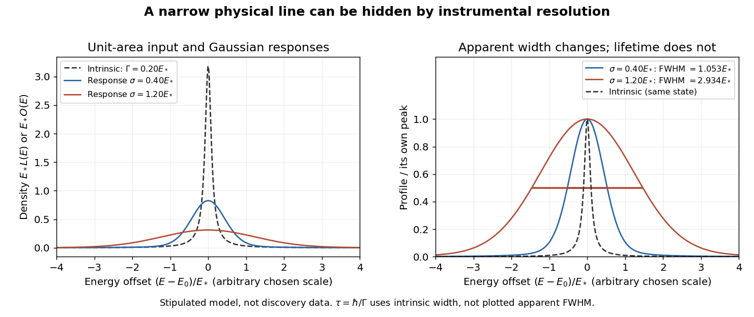
An arbitrary narrow line broadened by two stipulated Gaussian responses
. Original numerical convolution using a Lorentzian with intrinsic width 0.20 times an arbitrary energy scale and Gaussian standard deviations 0.40 and 1.20 times that scale. Left: densities with unit area on the whole line. Right: each profile divided by its own peak. No historical points, cross-section table or published curve were copied or fitted. Details.Choose an arbitrary scale , intrinsic decay width and response standard deviations and . Numerical integration gives apparent full width at half maximum values of approximately and , respectively. The state and its rest-frame lifetime are identical in both cases. The normal distribution's width alone is ; adding that width to in quadrature is not an exact rule for this convolution.
For a purely illustrative , taking gives . These are invented line parameters, not J/psi meson measurements. Substituting the larger apparent width into would incorrectly shorten the inferred lifetime by nearly a factor of fifteen. An unresolved width can support an upper bound on intrinsic decay width, and consequently a lower bound on lifetime, only after the instrumental response and model assumptions have been assessed.
The discovery peak and its later interpretation answer different questions. The J/psi meson is understood as charmonium, a bound charm quark–charm antiquark system. Richter's 1976 lecture distinguishes the initial discovery from subsequent tests of competing explanations, including the related level structure and later evidence for particles carrying uncancelled charm. A narrow peak alone did not establish all these properties in 1974.[ref]
From the Psi to Charm – The Experiments of 1975 and 1976 by Burton Richter. From the Psi to Charm – The Experiments of 1975 and 1976, introduction and sections 7.4–8: charmonium interpretation and subsequent charm searches
For a reconstructed electron–Positron pair, four-momentum conservation givesNeglecting the electron mass compared with the daughter energies, and calling the opening angle , this becomesAs an original example, choose , and . Then , although the pair's laboratory energy is . The pair carries net momentum. Neither its laboratory energy nor the original proton beam energy is its invariant mass; unobserved products carry additional four-momentum.
For equal, oppositely directed incoming beams with equal total energy , their total momentum vanishes. Thus the incoming center-of-mass energy isStipulated beams therefore provide of incoming center-of-mass energy. This identity is exact for the stated equal-beam geometry. Radiation before annihilation can reduce the energy forming the final state; the apparatus also has a distribution of beam energies. A nominal machine setting is therefore not an exact event-by-event final-state invariant mass.
At SPEAR, counterrotating electron and Positron beams collided inside a magnetic particle detector. Finer steps in stored-beam energy resolved a sharp production peak. A magnetometer and measured orbit positions monitored the energy settings; Bhabha scattering normalized the cross sections. The paper attributed the observed width to beam-energy spread and radiation effects, reporting an upper limit on intrinsic width. Its muon identification system was not functioning: the non-electron two-body excess was not conclusively a muon pair.[ref]
Discovery of a Narrow Resonance in e+e- Annihilation by J.-E. Augustin. Discovery of a Narrow Resonance in electron–positron Annihilation, pp. 1406–1408: scan, energy monitoring, normalization, width limit and two-body identification caveat
A scan must compare normalized production rates, since more selected events can result from more beam encounters or different detection efficiency. A proposed diagnostic is to revisit energies on either side of the peak while monitoring the energy calibration and event selection. Such neighboring settings test the local production background; their event totals alone are not an independent measurement of the intrinsic decay width.
Pinned article: Introduction to the OurBigBook Project
Welcome to the OurBigBook Project! Our goal is to create the perfect publishing platform for STEM subjects, and get university-level students to write the best free STEM tutorials ever.
Everyone is welcome to create an account and play with the site: ourbigbook.com/go/register. We belive that students themselves can write amazing tutorials, but teachers are welcome too. You can write about anything you want, it doesn't have to be STEM or even educational. Silly test content is very welcome and you won't be penalized in any way. Just keep it legal!
Intro to OurBigBook
. Source. We have two killer features:
- topics: topics group articles by different users with the same title, e.g. here is the topic for the "Fundamental Theorem of Calculus" ourbigbook.com/go/topic/fundamental-theorem-of-calculusArticles of different users are sorted by upvote within each article page. This feature is a bit like:
- a Wikipedia where each user can have their own version of each article
- a Q&A website like Stack Overflow, where multiple people can give their views on a given topic, and the best ones are sorted by upvote. Except you don't need to wait for someone to ask first, and any topic goes, no matter how narrow or broad
This feature makes it possible for readers to find better explanations of any topic created by other writers. And it allows writers to create an explanation in a place that readers might actually find it.
Figure 1. Screenshot of the "Derivative" topic page. View it live at: ourbigbook.com/go/topic/derivativeVideo 2. OurBigBook Web topics demo. Source. - local editing: you can store all your personal knowledge base content locally in a plaintext markup format that can be edited locally and published either:This way you can be sure that even if OurBigBook.com were to go down one day (which we have no plans to do as it is quite cheap to host!), your content will still be perfectly readable as a static site.
- to OurBigBook.com to get awesome multi-user features like topics and likes
- as HTML files to a static website, which you can host yourself for free on many external providers like GitHub Pages, and remain in full control

Figure 2. You can publish local OurBigBook lightweight markup files to either OurBigBook.com or as a static website.
Figure 3. Visual Studio Code extension installation.
Figure 5. . You can also edit articles on the Web editor without installing anything locally. Video 3. Edit locally and publish demo. Source. This shows editing OurBigBook Markup and publishing it using the Visual Studio Code extension. 
- Infinitely deep tables of contents:




All our software is open source and hosted at: github.com/ourbigbook/ourbigbook
Further documentation can be found at: docs.ourbigbook.com
Feel free to reach our to us for any help or suggestions: docs.ourbigbook.com/#contact