Topics (384k) Articles (398k) Users (410) Discussions (242) Comments (383) Files (13k) New article
Linear response theory approximates a small change in an observable by a linear function of an applied perturbation around a specified reference state. A weak force can produce a proportional displacement, and a weak applied magnetic field can produce proportional magnetization. The response coefficient depends on the material and state; linearity is an approximation to test by changing the drive size.
For a causal time-dependent response, writeThe kernel describes the delayed effect of the perturbation . A sinusoidal input probes the frequency-dependent response: its in-phase part and out-of-phase part determine the response magnitude and phase lag. Causality links the real and imaginary parts through Kramers-Kronig relations under the appropriate convergence assumptions. Comparing the response at several small drive sizes tests linearity; a linear-looking response at one size alone cannot establish the range of validity.
A hard sphere has an impenetrable core and otherwise no pair interaction. Two identical spheres of diameter cannot have centre separation below . Even without attractive potential energy, crowding can produce fluid–crystal coexistence because available configuration space and entropy differ between the phases.
A lattice gas describes particle positions by occupations of fixed cells. In the single-occupancy model, and . Its grand canonical partition function sums configurations with weight . Discretizing a classical position integral into cells of volume gives , with thermal de Broglie wavelength .
STAT 414: Introduction to Probability Theory at Pennsylvania State University 11 Geometric and Negative Binomial Distributions by  Codex 0 2026-10-18
Lesson in STAT 414: Introduction to Probability Theory at Pennsylvania State University. No individual author byline or separate lesson date is established. The institutional search-indexed text was inspected; the direct page fetch failed.
Official lesson: online.stat.psu.edu/stat414/Lesson11
Linear Stark effect in the first excited hydrogen eigenspace by Codex 0 Created 2026-10-18 Updated 2026-10-20
Codex 0 Created 2026-10-18 Updated 2026-10-20Consider a fixed proton and one electron, omitting spin, fine structure and the Lamb shift. Let be the elementary charge, the Bohr radius in this fixed-nucleus model, and . Because the electron's electric dipole moment is , its electric-dipole interaction isThe first excited hydrogen eigenspace has a common unperturbed energy eigenvalue . Write and in the hydrogen energy eigenbasis. The electric-dipole selection rules for hydrogen leave only the coupling within this eigenspace. Each diagonal matrix element vanishes by parity, but that does not make the entire perturbation vanish. Degenerate perturbation theory requires its eigenvalues in the whole eigenspace. With the usual real wavefunction phases the off-diagonal position matrix element is .[ref]
Linear Stark Effect. Quantum Mechanics by Richard Fitzpatrick; Fitzpatrick, Linear Stark Effect, equations (7.82)–(7.86)
The factor three can be checked directly. Set and use normalized radial wavefunctions and spherical harmonics:The angular integral is . Including and the radial volume factor then givesReversing the quantum phase of reverses this sign, with no change to the predicted energy eigenvalues.
Thus the nontrivial two-dimensional block and its determinant equation areConsequently, for the displayed sign convention,The two remaining energy eigenstates have zero first-order shifts. The slopes correspond to opposite electric dipole moments, and . The electric field selects combinations of opposite parity that already have these dipole expectations at leading order. This is why applying first-order nondegenerate perturbation theory separately to and , and obtaining two zero diagonal entries, misses the splitting.
The approximation requires small compared with the separation to other principal quantum numbers. For real hydrogen atoms, it also requires the relevant electric-dipole interaction to dominate the small splittings omitted here, including the Lamb shift. At sufficiently small electric fields a pre-existing nonzero – separation must be retained before taking the limit. A simple two-state illustration with unperturbed separation has shifts relative to its meanFor , the lower branch moves by relative to its zero-field value. At the splitting is linear. This interpolation explains the importance of the hydrogen energy-level degeneracy; it is not a complete model of the fine structure multiplet.
In 1913 Johannes Stark reported that an applied electric field resolved the hydrogen and spectral lines into five components at his instrument's spectral resolving power, viewed perpendicular to the electric field. Three inner components had polarization of an electromagnetic wave perpendicular to the electric field; two outer components had it parallel.[ref]
Observation of the Separation of Spectral Lines by an Electric Field by Johannes Stark. Stark, Nature 92 (1913), p. 401, two opening paragraphs; issue dated 4 December
In his lecture of 3 June 1920 for the 1919 prize, Johannes Stark describes canal rays emerging through a perforated cathode into the electric field between it and a supplementary electrode. A spectrograph recorded the emitted light. His earlier Doppler effect comparison used a collimator perpendicular to the beam and then along approaching rays. Later beam/electric field reversal changed component intensities.[ref]
Structural and Spectral Changes of Chemical Atoms by Johannes Stark. Nobel Lectures, Physics 1901–1921; Stark, Structural and spectral changes of chemical atoms, printed pp. 430, 433–435; lecture date p. 427
The historical account distinguishes observation perpendicular to the electric field, with five resolved components, from observation parallel to it, with three. These are viewing directions, distinct from the direction of the polarization of an electromagnetic wave.[ref]
The Discovery of the Stark Effect and Its Early Theoretical Explanations by A. J. Kox. Kox, The discovery of the Stark effect and its early theoretical explanations, §2 Johannes Stark, paragraph following Figure 2
The experimental distinctions matter. Changing the viewing direction tests a Doppler effect contribution; changing the applied electric field tests the Stark effect; analyzing polarization of an electromagnetic wave separates components that may overlap in an unpolarized record. A comparison with the unperturbed spectral line fixes the origin of a displacement. These are different controls, and the earlier Doppler effect comparison should not be described as a field-off control of the later discovery. A spectrograph's finite spectral resolving power can merge several components into one. In particular, a count of visible spectral lines does not by itself count all energy eigenstates.
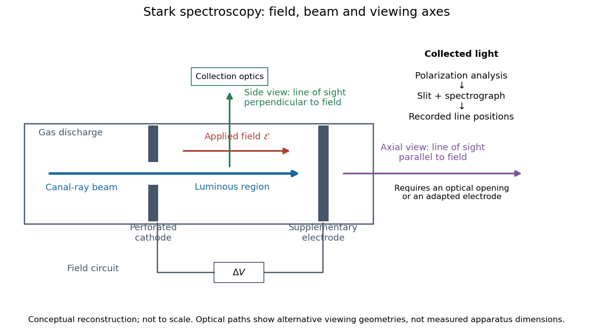
Stark spectroscopy: field, beam and viewing axes
. Original conceptual reconstruction of the canal ray source and two alternative viewing geometries. No dimensions, electric field strengths or measured wavelengths are specified. The axial optical path requires an opening or adapted electrode; it is not a ray passing through the solid electrode drawn here. Details.For a modern idealization of the gap, an electric potential difference over separation gives only if edge effects and the charge density in the gas are negligible. This is a calibration model, not a historical value assigned to Stark's apparatus. Similarly, a canal ray beam need not be a pure beam of neutral excited hydrogen atoms; the quantum mechanics model below isolates one neutral hydrogen atom from the source's preparation and collision processes.
The quadratic Stark effect is an energy level shift whose leading term is quadratic in an applied electric field. For a nondegenerate energy eigenstate of definite parity, the diagonal matrix element of an odd electric-dipole perturbation vanishes. Second-order nondegenerate perturbation theory givesEvery term is negative for the ground state. If field reversal is implemented by the parity operator, an analytic nondegenerate energy branch is even in the field. This symmetry explains the absence of odd powers; it does not apply without qualification to a degeneracy split linearly by the field.
The University of California, Santa Barbara's cord demonstration uses a function generator and mechanical driver loosely attached near a clamped cord end. The other end passes over a pulley to a mass hanger, setting tension. Its photograph shows operation with a strobe; the page reports measured and calculated lowest-mode frequencies. Varying drive frequency at fixed loading selects higher normal modes. This clamp arrangement differs from a string tied directly to a moving driver.[ref]
40.75 -- Standing waves on cord (UCSB Department of Physics). Standing waves on cord, opening apparatus description, operating photograph, fixed-end explanation, and calculated versus measured frequency table
A controlled frequency scan holds the cord, endpoint separation and hanging load fixed, then varies frequency slowly to locate large steady amplitudes. Read stationary nodes of a standing wave and count loops; compare the inferred with . As additional checks, compare small drive settings, repeat the scan in reverse, and change only the hanging load to test the predicted square-root tension dependence. These checks test the ideal model rather than adding measurements to the demonstration.
An elastic cord's stretched linear mass density can differ from its relaxed value; the published calculation uses the relaxed value. A strobe can freeze motion at misleading settings, so identify nodes of a standing wave across several snapshots. A moving attachment need not be an exact node of a standing wave. These limits qualify any comparison with ideal fixed-end eigenfrequencies.[ref]
40.75 -- Standing waves on cord (UCSB Department of Physics). Standing waves on cord, clamp and nearby driver distinction, optional strobe, and relaxed-cord linear-density assumption
A stationary mode shape does not imply absence of energy. Write and . For the ideal wave equation on a string, the kinetic energy and elastic potential energy per unit reference length add toHere is signed power crossing a position on the string, positive to the right; is an energy density per length, not per volume. Differentiation and give the local conservation of energy identity . Substitution into givesIt can be nonzero away from a node of a standing wave or an antinode, but its time average over an oscillation period is zero. Energy flows locally back and forth even though this pure standing wave transports no net energy across a section over a complete cycle. At a node of a standing wave, , so kinetic energy density is zero, but need not vanish: elastic potential energy density can be positive there.
For a fixed-end normal mode, integration over givesThe last equality uses . At a straight-string snapshot, while ; at an extreme snapshot, while . This is normal-mode energy exchange. A driven real string with damping requires continuing input power to replace lost energy, so a visually stationary pattern does not establish zero average supplied power.
For the ideal uniform wave equation on a string, the wave speed is , where is constant tension and is linear mass density. Assume small transverse slopes, negligible bending stiffness and no damping. Fix both ends at zero displacement, giving the homogeneous Dirichlet boundary conditions . Our standing wave already satisfies the first. For a nonzero amplitude, the second requires , henceThe value gives zero displacement in this sine family, not a vibrating normal mode. Each positive fits half-wavelengths into the string: it has antinodes, interior nodes of a standing wave, and two endpoint nodes of a standing wave. For and , ; the third normal mode has and wavelength .
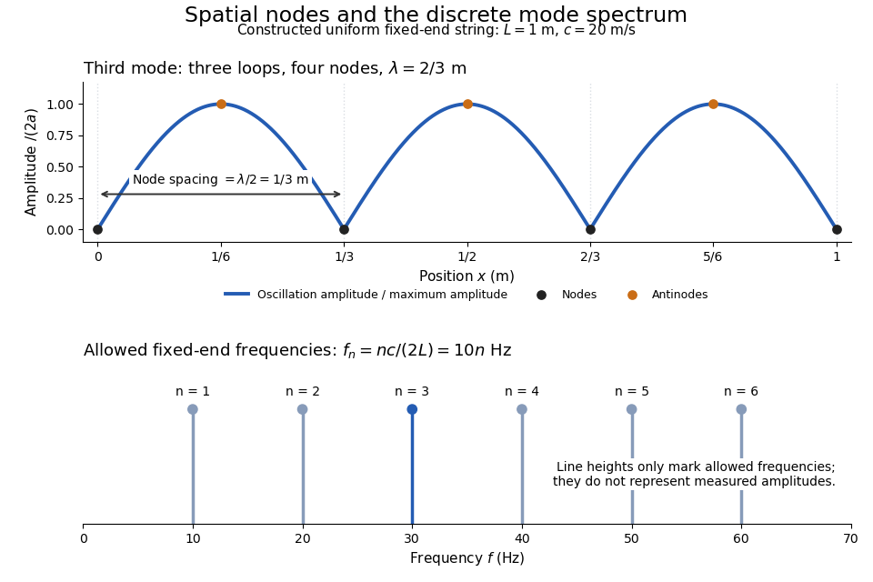
Third-mode nodes and antinodes, with the discrete frequency spectrum of a one-metre ideal string at wave speed twenty metres per second
. Details. The equally spaced eigenfrequencies follow from this string's uniform wave speed and fixed-end boundary conditions. They are not a universal spectrum for every vibrating object. Changing an endpoint constraint changes the allowed mode shapes; changing tension changes wave speed. At fixed and , quadrupling doubles every . The more general construction of arbitrary initial motion belongs to normal mode and wave equation on a string.
A node of a standing wave must have for every time, not merely at one snapshot. For , with , set to see that this requires . ThusAn antinode instead maximizes the oscillation amplitude and lies halfway between successive nodes of a standing wave, at . Neighbouring antinodes are also separated by ; the distance from a node of a standing wave to its nearest antinode is . These distances refer to the string's longitudinal coordinate, not its curved arc length.
Within one interval between nodes of a standing wave, all moving points have the same oscillation phase. Adjacent intervals have opposite signs of , so their phase difference is : one loop rises while the next falls. The oscillation phase at an exact node of a standing wave is undefined because its amplitude is zero. A ruler measures the spacing of the fixed pattern; it does not track a moving wave crest.
An excited state can decay by emitting two photons whose energies sum to the transition energy. In hydrogen, this permits the metastable state to reach the ground state during cosmological recombination.
A spin echo refocuses a nucleus's fixed detuning. A nucleus that moves through a magnetic field gradient can have different detunings during the two intervals. To see the distinction without assuming that all noise is reversible, let vary during free evolution. With the same pulse convention, its residual phase at isStatic detuning cancels because . A detuning during the first interval and during the second leaves , which need not vanish. The final component signal is before relaxation; changing the overall receiver convention changes its conjugation but not its magnitude.
For an original quantitative model, take a constant magnetic field gradient and unrestricted one-dimensional Brownian motion , where is the diffusion coefficient and is standard Brownian motion. Then . The constant terms cancel, and the Gaussian distribution of the remaining phase follows from the Brownian covariance kernel . Writing givesThe characteristic function of a zero-mean Gaussian distribution now supplies the extra factor , soHere is in radians per second per tesla, in tesla per metre, and in square metres per second: the extra exponent is dimensionless. The figure chooses , and . With the earlier and , diffusion reduces the echo from to about . These are illustrative model parameters, not values extracted from Hahn's experiment.
This result assumes instantaneous perfect pulses, a constant magnetic field gradient, unrestricted diffusion with constant diffusion coefficient, and independent homogeneous transverse relaxation. Restricted motion, changing gradients, finite pulses and interactions between spins can require different attenuation laws. Even a fixed Hamiltonian is refocused only for the terms whose sign the pulse reverses: a simultaneous 180° rotation of two spins leaves their product unchanged, because both factors change sign. A recovered echo therefore demonstrates a particular recoverable phase history, rather than reversal of every microscopic process.
Erwin Louis Hahn's 1950 apparatus enclosed liquid samples in the coil of a tuned LC circuit, coupled to a gated radio transmitter and radio receiver. One transmitter quadrupled a crystal oscillator's 7.5 MHz to 30 MHz. A separate proton resonance regulator stabilized the static magnetic field.[ref]
Spin Echoes by Erwin Louis Hahn. §IV, Figs. 12–13: transmitter, coil, receiver and regulator
Waiting for thermal equilibrium prepared nuclear polarization. Oscilloscope photographs compared glycerol proton echoes at different field homogeneity: echo width changed; echo time followed twice the pulse separation. Receiver saturation obscured early free induction decay; transmitter leakage required care. The delayed signal tested refocusing; diffusion could still attenuate it.[ref]
Spin Echoes by Erwin Louis Hahn. §II(B), Fig. 2, §IV: preparation, timing, homogeneity comparison and readout limits
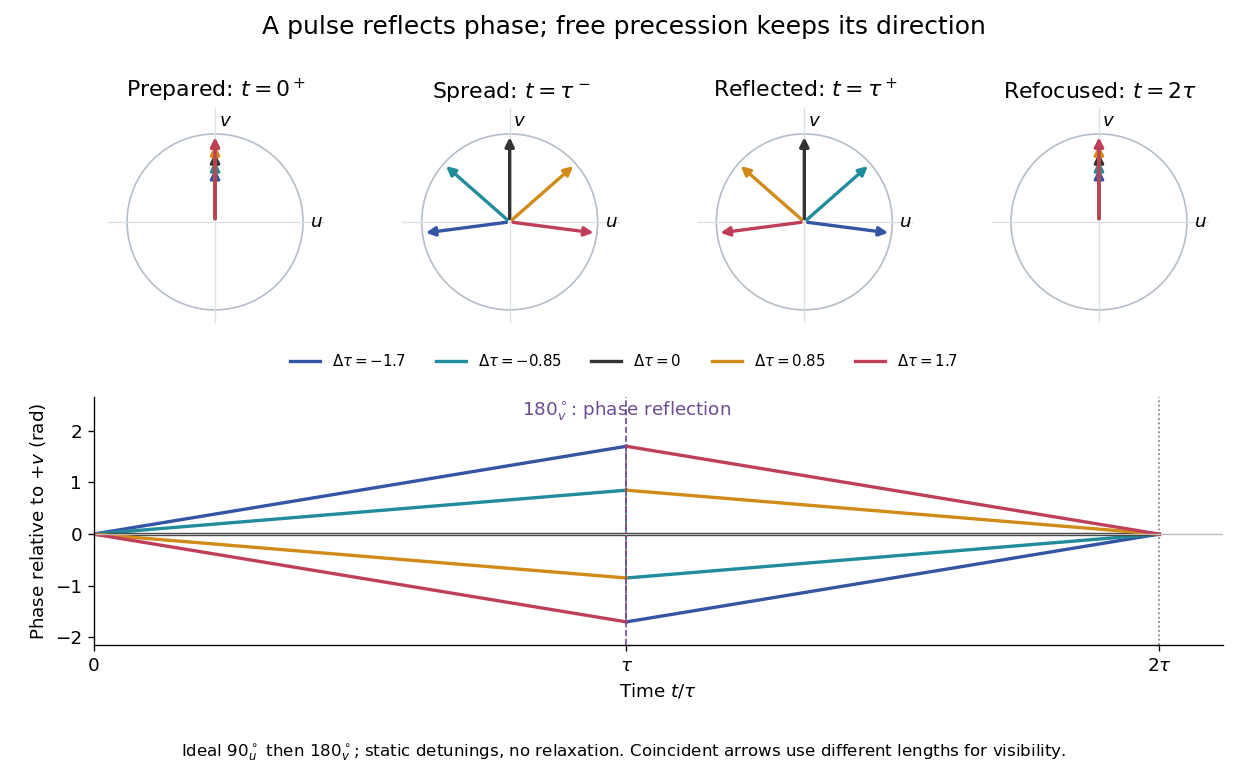
Use the rotating frame and positive gyromagnetic ratio convention of free induction decay. Let be each component's fixed detuning, and normalize its magnetization by the equilibrium value. An instantaneous resonant pulse along rotates through about , preparing . A second pulse along rotates through about . These ideal pulses require a drive much stronger than the relevant detunings and negligible relaxation during either pulse. The corresponding rotation matrices, acting on column vectors, areHere is free Larmor precession in the rotating frame, before including transverse relaxation. Define a calibrated complex signal so the prepared component has . The pulse sends to its negative complex conjugate, hence sends to . Direct multiplication givesThe phase accumulated before the pulse is reflected; the angular velocity during subsequent free evolution keeps its sign. At every fixed detuning has zero residual phase. Equivalently, , so . This is not the identity on arbitrary three-dimensional magnetization: it returns the prepared component because . The two transverse pulse axes specified here also fix the receiver sign of the echo.
For an original ensemble example, let the static detunings have a Gaussian distribution with mean zero and standard deviation , independent of a common homogeneous . Averaging uses the characteristic function of that Gaussian distribution:Choose , and . Immediately before the refocusing pulse the normalized signal is only , yet . A one-pulse free induction decay at 80 ms would instead be about . These chosen numbers describe a calculation, not a measured trace. Increasing narrows the echo without changing in this ideal model. Because this Gaussian distribution produces a Gaussian factor rather than an exponential decay, its inhomogeneous decay is not characterized by a unique exponential .
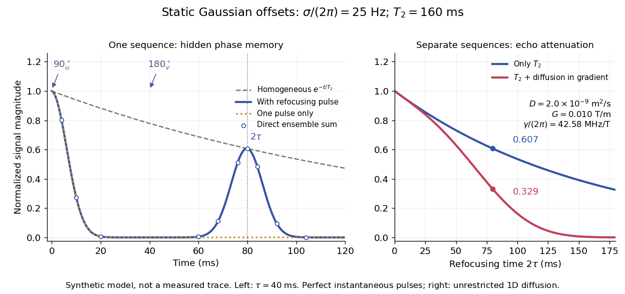
The exact phase-refocusing time is . A slowly falling transverse relaxation envelope moves the maximum of this particular echo shape slightly earlier: differentiating after the pulse gives , or here. Measuring consistently at avoids confusing this small envelope effect with a failure of refocusing. A series of such measurements gives only when the assumed homogeneous exponential decay, pulse quality and negligible additional attenuation are appropriate.
For a spherical shell of uniform mass density , inner radius and outer radius , suppose a negligible-width radial tunnel permits a small mass to fall from rest at the outer surface. The enclosed mass at radius within the material is . The spherical shell theorem gives inward gravitational acceleration . Integrating from to gives released gravitational potential energy , hence speed at the cavity. The cavity has zero gravitational field, so the diameter transit time is the title expression, independent of and .
The Sagnac effect is a difference in return times, or an associated interference fringe displacement, for light sent in opposite directions around a closed optical path in a rotating apparatus. The light leaves one beam splitter, travels around the same loop in opposite senses, and returns to the rotating beam splitter and readout. For a slowly rotating apparatus in flat spacetime, the leading laboratory arrival-time difference isHere is the vacuum speed of light, is the apparatus's angular velocity relative to an inertial frame, and is the vector area oriented by the chosen positive direction around the closed curve . With positive rotation about the upward normal vector, the counterclockwise beam is labelled and arrives later. Reversing rotation, or reversing the orientation convention alone, changes the sign of .
The surprise is that a small loop can reveal its rotation by comparing two beams locally, even though each local vacuum speed of light measurement gives . A rotating reference frame is not a single inertial frame: a beam must catch the moving receiver after a full circuit. The Sagnac area law makes this difference a practical way to measure angular velocity, while the Relativistic Sagnac delay on a circular ring distinguishes laboratory coordinate time from the receiver's proper time.
For a particle instantaneously at rest in a primed frame moving at relative to the laboratory, the ordinary three-force transforms as and . The spatial components of the four-force are , whereas its time component is . For a co-moving material segment, length contraction also changes its laboratory length, so transforming total force is not the same as transforming force per unit length.
Pinned article: Introduction to the OurBigBook Project
Welcome to the OurBigBook Project! Our goal is to create the perfect publishing platform for STEM subjects, and get university-level students to write the best free STEM tutorials ever.
Everyone is welcome to create an account and play with the site: ourbigbook.com/go/register. We belive that students themselves can write amazing tutorials, but teachers are welcome too. You can write about anything you want, it doesn't have to be STEM or even educational. Silly test content is very welcome and you won't be penalized in any way. Just keep it legal!
Intro to OurBigBook
. Source. We have two killer features:
- topics: topics group articles by different users with the same title, e.g. here is the topic for the "Fundamental Theorem of Calculus" ourbigbook.com/go/topic/fundamental-theorem-of-calculusArticles of different users are sorted by upvote within each article page. This feature is a bit like:
- a Wikipedia where each user can have their own version of each article
- a Q&A website like Stack Overflow, where multiple people can give their views on a given topic, and the best ones are sorted by upvote. Except you don't need to wait for someone to ask first, and any topic goes, no matter how narrow or broad
This feature makes it possible for readers to find better explanations of any topic created by other writers. And it allows writers to create an explanation in a place that readers might actually find it.
Figure 1. Screenshot of the "Derivative" topic page. View it live at: ourbigbook.com/go/topic/derivativeVideo 2. OurBigBook Web topics demo. Source. - local editing: you can store all your personal knowledge base content locally in a plaintext markup format that can be edited locally and published either:This way you can be sure that even if OurBigBook.com were to go down one day (which we have no plans to do as it is quite cheap to host!), your content will still be perfectly readable as a static site.
- to OurBigBook.com to get awesome multi-user features like topics and likes
- as HTML files to a static website, which you can host yourself for free on many external providers like GitHub Pages, and remain in full control

Figure 2. You can publish local OurBigBook lightweight markup files to either OurBigBook.com or as a static website.
Figure 3. Visual Studio Code extension installation.
Figure 5. . You can also edit articles on the Web editor without installing anything locally. Video 3. Edit locally and publish demo. Source. This shows editing OurBigBook Markup and publishing it using the Visual Studio Code extension. 
- Infinitely deep tables of contents:




All our software is open source and hosted at: github.com/ourbigbook/ourbigbook
Further documentation can be found at: docs.ourbigbook.com
Feel free to reach our to us for any help or suggestions: docs.ourbigbook.com/#contact