Topics (384k) Articles (398k) Users (410) Discussions (242) Comments (383) Files (13k) New article

The Pearson chi-squared test compares observed categorical counts with null expected counts using the displayed statistic. Its applications include Pearson chi-squared goodness-of-fit test for specified probabilities and Pearson chi-squared test of independence for contingency tables; the fitted restrictions determine the limiting degrees of freedom.
For paired binary observations , let count pairs and pairs . Under the null hypothesis of equal marginal event probabilities, these discordant outcomes have equal probabilities. Conditional on , has the binomial distribution , giving an exact test. For enough discordant pairs, has an approximate standard normal distribution, or its square has an approximate one-degree-of-freedom chi-squared distribution. Concordant pairs provide no information about the direction of the marginal difference. If there are no discordant pairs, there is no directional information and the divided statistic is not computed. The pairing and independence between pairs are essential; the usual independent-two-sample formula is not a paired test.
A rejection region is the set of sample outcomes on which a hypothesis test rejects its null hypothesis. Its probability under the null determines the type I error rate.
For independent multivariate normal observations with positive-definite covariance, this statistic is the maximum squared studentized mean contrast. With unbiased sample covariance matrix and , its null distribution obeys . This follows from independence of the Gaussian sample mean and the residual Wishart distribution.
The alternative hypothesis specifies the parameter values or distributions against which a null hypothesis is tested. If the null is , the alternative is with . For example an upper one-sided comparison uses , while a two-sided comparison uses . The alternative determines the relevant rejection tail. A p-value is computed under the null; it is not the probability that the alternative is false.
A one-sided test targets deviations in one specified direction, such as . If larger values of a statistic indicate this direction, its p-value is an upper-tail null probability . The direction should be chosen from the scientific question before examining the data. An upper normal test uses ; a lower test uses .
A two-sided test detects departures in either direction from the null hypothesis, for example . With a continuous symmetric null statistic centred at zero, its p-value is . This is the usual coefficient test printed by Gaussian regression summaries, unlike a directional one-sided comparison.
A result is statistically significant at a specified significance level when its valid p-value is at most and the corresponding null hypothesis is rejected. Significance does not measure effect size, establish practical importance, or give the probability that the null is true. Software stars encode thresholds for -values; they do not supply an additional statistic.
A sequential probability ratio test accumulates the log-likelihood ratio for two specified simple statistical hypotheses until it reaches an upper or lower boundary. An upper crossing favors the alternative, a lower crossing favors the null, and observations continue between them. Error-calibrated boundaries are approximately and ; discrete overshoot means these approximations need calibration.
A statistical hypothesis is a specified set of possible data-generating probability distributions, usually expressed as a restriction on model parameters. A simple statistical hypothesis specifies one distribution; a composite statistical hypothesis permits several. A hypothesis test compares a null hypothesis with an alternative hypothesis using a statistic calibrated under the null.
The periodic second-difference circulant matrix has constant null space, so solvability requires . Its Jacobi method has eigenvalues : for odd it converges to some solution, while for even an alternating mode oscillates unless absent from the error. Lexicographic Gauss-Seidel iteration converges to some solution for every compatible right-hand side and every initial vector. For , a coordinate sweep decreases the energy by the sum of squared coordinate changes. This excludes all nonconstant unit-modulus eigenmodes. The constant unit eigenvalue is simple, since the invariant left vector has . Neither method is a strict contraction to a unique solution without fixing the constant nullspace.
For a primary operator, . Taking the residue against gives the weight for , the derivative descendant for , and zero for every . Conversely the absence of positive-mode actions excludes higher poles in this operator product and gives the primary transformation law. The antiholomorphic argument is identical. Thus primary states and primary operators correspond under radial quantization.
A linear subalgebra closed under the involution. In bounded operators, this means closure under the adjoint operator; neither norm closure nor operator-topology closure is part of the definition. These distinctions matter in the Von Neumann double commutant theorem and the Kaplansky density theorem.
A Hermitian algebra element of a star-algebra is an element fixed by its algebra involution. The identity and zero are Hermitian algebra elements. For every , both and are Hermitian algebra elements. A real spectrum for all such elements is an extra condition in a general Banach algebra, rather than a consequence of the involution identities alone.
In one Standard Model generation, the left-handed up and down quark fields form a weak doublet of hypercharge . Each weak component has three colours. The same field therefore counts as three doublets for weak gauge-loop contributions and two colour fundamentals for strong gauge-loop contributions. Right-handed up and down quarks are separate weak singlets.
The stalk supporting an anther.
The Gale-Shapley algorithm constructs a stable matching by letting one side propose and the other hold its best offer so far. The word "deferred" is essential: a held proposal is tentative and can be replaced. David Gale and Lloyd Shapley presented this construction in their 1962 paper, College Admissions and the Stability of Marriage, §3, printed pp. 12–13; §4 extends it to college quotas and unacceptable pairs.
For the one-partner bipartite graph model, designate as proposers and as receivers:
- Start with the empty matching in a graph. Each proposer keeps a pointer to its first untried acceptable partner.
- Choose an unmatched vertex in a matching whose list is not exhausted. It proposes to its highest-ranked untried neighbour of a vertex and advances its pointer permanently.
- If holds nobody, it holds . Otherwise compares with its currently held proposer, keeps the one it prefers, and rejects the other. A displaced proposer becomes unmatched and may propose again later.
- Stop when every unmatched proposer has exhausted its list. The held pairs are the output matching in a graph.
Held proposers wait; only unmatched proposers act. A receiver can replace its held partner, whereas a proposer never tries the same edge twice. Isolated vertices simply remain unmatched. These rules also describe incomplete acceptable lists and unequal sides without adding fictitious acceptable partners.
For the preference lists under stable matching, choose available proposers in queue data structure order, initially , adding rejected proposers at the end. The proposals are , , , , . At the fourth proposal, replaces its held by because . This frees to try , producing .
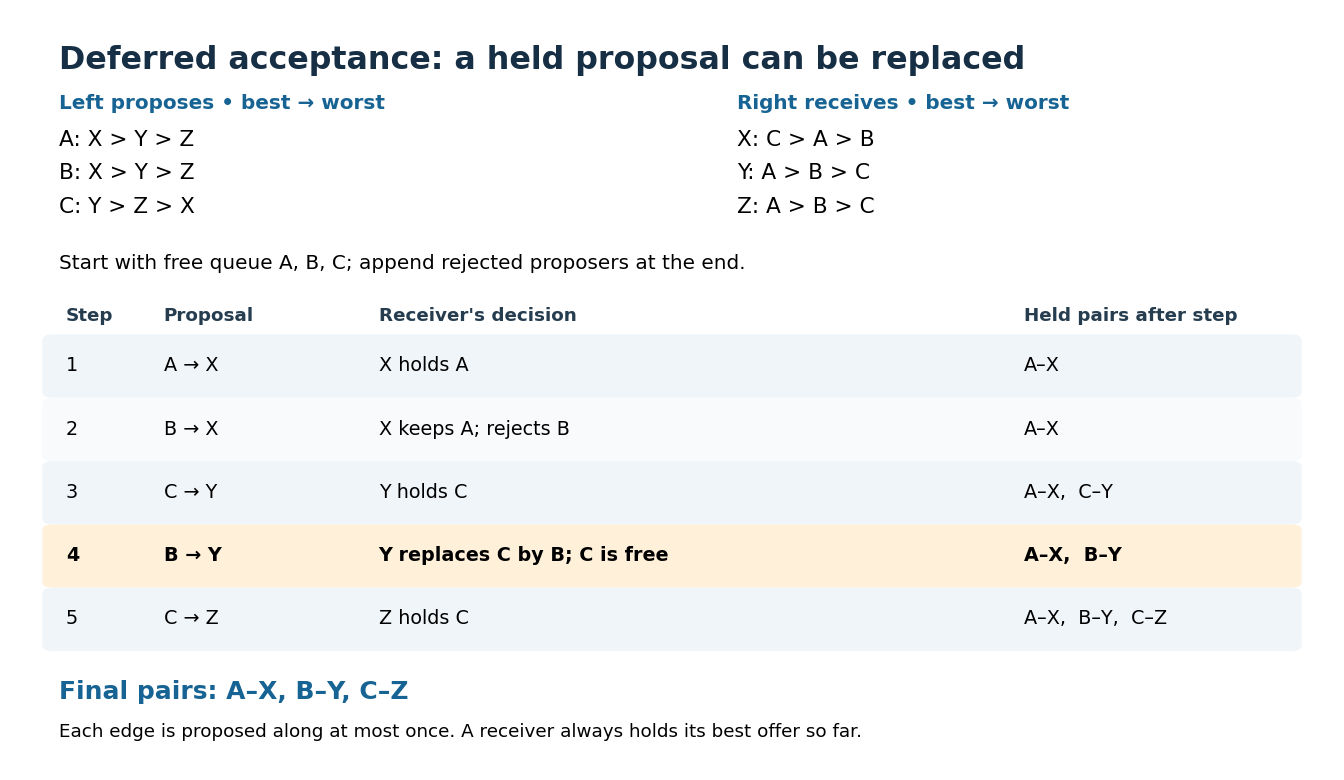
Five proposals in the Gale-Shapley algorithm: Y replaces a tentative partner before the final stable matching
. Details. Reverse the proposing side. Starting in the order , the proposals are , , , . Now rejects because it already holds . The result is . Thus the choice of proposing side can change the output even with strict preferences and complete lists.
Why does the procedure work? Each edge receives at most one proposal, so at most proposals occur. At all times, the held edges form a matching in a graph, and each receiver holds its favourite proposer among all proposals received. A receiver's held partner can only improve according to its strict preference. If a proposer prefers to its final partner, or ends unmatched while is acceptable, it must already have proposed to . A rejection means then held someone better, and its final partner is at least as good. Such an edge cannot be a blocking pair in stable matching. This covers every possible blocking pair in stable matching, proving stability at termination.
With a queue data structure of unmatched proposers, a next-choice pointer for each list, and constant-time receiver-rank lookups, each proposal takes constant work. Using Big O notation, the time complexity is including initialization, provided list construction and rank preprocessing also take . Edge-indexed ranks with cross-referenced list entries, or expected constant-time hash lookups, allow sparse storage proportional to . Repeatedly scanning a receiver's preference list to compare offers would lose this bound. For complete lists with vertices per side, and the bound is . Initializing full rank tables itself costs time and space, even when only a sparse set of pairs is acceptable.
The Gale-Shapley algorithm does more than establish existence: with strict preferences, its output is a proposer-optimal stable matching.[ref]
College Admissions and the Stability of Marriage by David Gale and Lloyd Shapley. §5, printed p. 14, Theorem 2: applicant optimality and the rejection induction
It is also a receiver-pessimal stable matching, as proved below. Both qualifications compare partners across stable matchings.If the endpoints of an edge rank one another last and one stable matching in a bipartite graph contains that edge, every stable matching contains it. In the symmetric difference of two stable matchings, preference comparisons propagate along alternating paths: if a vertex prefers its new partner, that partner must prefer its old partner to avoid blocking the old matching. An alternating path cannot end unmatched on the preferred side, so the component is an alternating cycle, on which the two parts prefer opposite matchings. A mutual-worst edge absent from the new matching would make both its endpoints prefer the new matching, contradicting this propagation.
Pinned article: Introduction to the OurBigBook Project
Welcome to the OurBigBook Project! Our goal is to create the perfect publishing platform for STEM subjects, and get university-level students to write the best free STEM tutorials ever.
Everyone is welcome to create an account and play with the site: ourbigbook.com/go/register. We belive that students themselves can write amazing tutorials, but teachers are welcome too. You can write about anything you want, it doesn't have to be STEM or even educational. Silly test content is very welcome and you won't be penalized in any way. Just keep it legal!
Intro to OurBigBook
. Source. We have two killer features:
- topics: topics group articles by different users with the same title, e.g. here is the topic for the "Fundamental Theorem of Calculus" ourbigbook.com/go/topic/fundamental-theorem-of-calculusArticles of different users are sorted by upvote within each article page. This feature is a bit like:
- a Wikipedia where each user can have their own version of each article
- a Q&A website like Stack Overflow, where multiple people can give their views on a given topic, and the best ones are sorted by upvote. Except you don't need to wait for someone to ask first, and any topic goes, no matter how narrow or broad
This feature makes it possible for readers to find better explanations of any topic created by other writers. And it allows writers to create an explanation in a place that readers might actually find it.
Figure 1. Screenshot of the "Derivative" topic page. View it live at: ourbigbook.com/go/topic/derivativeVideo 2. OurBigBook Web topics demo. Source. - local editing: you can store all your personal knowledge base content locally in a plaintext markup format that can be edited locally and published either:This way you can be sure that even if OurBigBook.com were to go down one day (which we have no plans to do as it is quite cheap to host!), your content will still be perfectly readable as a static site.
- to OurBigBook.com to get awesome multi-user features like topics and likes
- as HTML files to a static website, which you can host yourself for free on many external providers like GitHub Pages, and remain in full control

Figure 2. You can publish local OurBigBook lightweight markup files to either OurBigBook.com or as a static website.
Figure 3. Visual Studio Code extension installation.
Figure 5. . You can also edit articles on the Web editor without installing anything locally. Video 3. Edit locally and publish demo. Source. This shows editing OurBigBook Markup and publishing it using the Visual Studio Code extension. 
- Infinitely deep tables of contents:



All our software is open source and hosted at: github.com/ourbigbook/ourbigbook
Further documentation can be found at: docs.ourbigbook.com
Feel free to reach our to us for any help or suggestions: docs.ourbigbook.com/#contact