Topics (384k) Articles (398k) Users (410) Discussions (242) Comments (383) Files (13k) New article

A harmonic majorant of a real function is a real harmonic function with pointwise. A least harmonic majorant lies below every other harmonic majorant. A continuous subharmonic function need not have one: on the unit disk has increasing circular means diverging to infinity, whereas any harmonic majorant would have the same finite mean on every centered circle.
Write a holomorphic function as . The Cauchy-Riemann equations make harmonic functions and give , . The product rule therefore gives . Thus its squared modulus is subharmonic and is harmonic only where vanishes.
For every holomorphic function and , is subharmonic. Away from its zeros the displayed Laplacian calculation proves this. At the zeros, use the smooth approximations , whose Laplacians are nonnegative, and let in their mean inequalities. This permits Poisson integral comparison for fractional modulus powers even when a global analytic fractional power does not exist.
For a specified subgroup and a chosen alphabet for , the membership problem asks whether an input word represents an element of . Solubility of the ordinary word problem for a group does not imply solubility of this problem, even for finitely generated subgroups: a Mihailova subgroup of a product of finite-rank free groups can have undecidable membership.
A subgroup is finitely generated when finitely many of its elements generate it as a group. Even inside a finitely generated group, subgroups need not be finitely generated. Finite generation of a witness subgroup, rather than of the original intersection, is what makes centralizing HNN extensions usable for a benign subgroup.
A real convex function locally bounded on an open convex set has a continuous supporting linear functional at every interior point. Apply the dominated Hahn-Banach theorem to its sublinear directional derivative to obtain . Increasing secant slopes imply whenever the endpoint is in the domain. A local Lipschitz continuity bound gives both and , proving continuity.
Loop subdivision refines an interior triangular mesh by splitting each face into four triangles and updating control points with local affine combinations. For an old vertex with cyclic neighbors , the original vertex rule isFor an interior edge with endpoints and opposite triangle vertices , the new edge vertex isOn the regular triangular lattice , , so . The coefficient sums are one, giving affine equivariance of a geometric basis; their nonnegativity also gives a convex hull bound. These are interior rules: a boundary or a deliberately retained sharp crease needs its own specified stencil.
The scheme is approximating rather than interpolatory. If an old vertex has height one and its six regular neighbors have height zero, its new height is , so refinement moves the old vertex. On regular patches the limit is a quartic box spline; extraordinary subdivision vertices require the local subdivision matrix and characteristic map of a subdivision surface analysis. The method is named for Charles Loop, whose 1987 thesis introduced the triangular scheme.[ref]
Convex Triangular Subdivision Surfaces with Bounded Curvature by Charles Loop. Section 2, original masks; section 4, Remark 1 and constraint summary: original central weight and subdominant eigenvalues
[ref]Smooth Subdivision Surfaces Based on Triangles by Charles Loop. Official publication record: thesis title, author and 1987 date
// Target: analysis.bigb
A regular quincunx subdivision step replaces a square lattice by the union of its old vertices and face centres. In lattice indices one may useThus two steps give ordinary binary refinement. If is the one-step subdivision mask symbol, the two-step symbol is . The two lattice parity classes separately determine the old-vertex and face-vertex stencils; their coefficient sums must each be one to reproduce constants.
An extraordinary subdivision vertex has a valence different from that of the regular refinement lattice. Regular box spline calculations do not alone establish smoothness at this vertex. The finite local subdivision matrix, its eigenvalues, and the associated characteristic map of a subdivision surface determine convergence and tangent behavior.
Interrogation of a subdivision limit needs patch/topology navigation, refinement, limit evaluation and derivatives where they exist, with certified bounds and geometric error estimates. On regular patches one may use the corresponding spline representation. At extraordinary subdivision vertices, local subdivision matrices determine limit positions and tangents under the scheme's smoothness conditions. A normal vector may exist even when second derivatives and Gaussian curvature do not; finite refined polygons are approximations rather than exact limit queries.
Mid-edge subdivision replaces each mesh edge by its midpoint, joins successive midpoints around every old face, and joins successive midpoints around every old vertex. For an interior manifold mesh, each new vertex has valence four. Each geometric update is a convex combination, so every refined control point remains in the convex hull of the original control mesh. The regular limit is associated with the quadratic four-direction box spline.
Lateral artifacts of a subdivision surface are unwanted variations along an intended straight extrusion: input cross-sections identical along a lattice direction acquire ripples in that direction under refinement. For a stationary arity- lattice rule , extrusion along the first lattice coordinate is preserved exactly when is independent of the residue for every transverse offset . Then summing along each row gives a single associated univariate subdivision mask. This direction-specific criterion does not promise invariance under every possible oblique extrusion.
A useful subdivision curve interface provides parameter ranges, endpoint and limit evaluation, derivatives, subdivision into equivalent restricted pieces, a certified bounding volume, and a certified error relative to a chord. Positive subdivision masks often give a convex hull bound. Masks with negative coefficients need a separate enclosing bound; their control-point hull need not enclose the limit curve.
Under , the descendants of control index zero lie at , where each is in the mask support. Dividing by the refined parameter scale gives a limiting influence enclosure with the displayed endpoints. For a mask supported on its width is when the endpoints are active and a nonzero compactly supported basic limit exists. To prove exactness, the largest active mask term is the only surviving term near the right endpoint of the refinement equation, forcing ; the analogous left-end argument completes the result. Mask padding should be removed, and a nonconvergent rule has no limit support.
Chaikin subdivision generates a rounded subdivision curve by repeatedly cutting the corners off a control polygon. Each edge contributes two new control points, one a quarter of the way along the edge and the other three quarters of the way along it. Connecting these new control points in edge order replaces the old corners by shorter line segments. This makes Chaikin subdivision a useful way to draw a smooth outline from a small, editable set of control points, without evaluating B-spline basis functions at each drawing step. Joy presents both the corner-cutting rule and its closed version.[ref]
https://www.cs.unc.edu/~dm/UNC/COMP258/LECTURES/Chaikins-Algorithm.pdf. Kenneth I. Joy, Chaikin's Algorithms for Curves, §§Chaikin's Method and Example — A Closed Curve, UC Davis authored notes
For a closed control polygon with control points , set and interpret indices cyclically. One refinement givesand the new control polygon is the ordered sequenceClose it by joining back to . Use the old control points for every average in the same refinement; updating them in place would define a different algorithm. One refinement produces stored control points, and refinements produce , counting entries even if some coordinates coincide. Open control polygons need an explicit endpoint convention: applying only the interior edge rule discards the original endpoints, whereas retaining endpoints changes the boundary rule. The closed analysis below uses cyclic indices throughout.
For a worked example, start with the rectangular control polygonThe first edge gives and . Applying Chaikin subdivision to all four edges, including the closing edge, gives exactly eight control points in this order:Thus the rectangle becomes an octagonal control polygon. Two refinements have control points, and five have . The illustration shows finite control polygons at stages ; the last is already visually rounded but still consists of line segments.
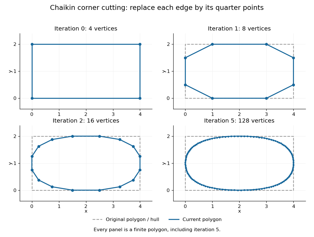
The convex hull property follows directly from the weights. Each new control point is a convex combination of the endpoints of one old edge, because the weights are nonnegative and sum to one. Consequently, if is the convex hull of the stage- control points, then . Every later line segment, and every limit point, stays in the original convex hull. This gives a useful geometric enclosure. It also explains why Chaikin subdivision is approximating rather than an interpolation rule: the rectangle's four original corners are outside the first octagon's convex hull, so the limiting curve cannot pass through them. A refinement control polygon generally lies off the limiting curve as well.
For the cyclic uniform rule, the closed limit is the periodic quadratic uniform B-spline curve determined by the original control points. Uniform refers to equal spacing in the spline knot sequence, not equal physical lengths of edges of the control polygon. An infinite uniform control sequence has the corresponding local description; arbitrary open endpoint conventions need separate treatment. Joy derives the quarter-point refinement by splitting quadratic uniform B-spline spans.[ref]
https://www.cs.unc.edu/~dm/UNC/COMP258/LECTURES/Quadratic-B-Spline-Curve-Refinement.pdf. Kenneth I. Joy, Quadratic Uniform B-Spline Curve Refinement, §§Splitting and Refinement and The General Refinement Procedure, UC Davis authored notes
Here is an explicit description of that closed limit, with cyclic indices and a unit parameter span for each original control point:Each coordinate is a quadratic polynomial, and the three coefficients form a nonnegative partition of unity. The span runs from to . Differentiating gives and , so adjacent spans have matching values and matching first derivatives. Their second derivatives generally differ. Thus the parameterized curve is , generally not ; degenerate control points can still make its tangent vector vanish. For the rectangle, the span around iswhich rounds the original corner between edge midpoints and . For equally spaced abscissae, the centered Chaikin basis function gives the scalar graph version of this quadratic B-spline representation and has support of width three original grid intervals.
Another useful property is affine equivariance of a geometric basis: refining and applying an affine map commute. For ,and the same calculation holds for . The sum-to-one weights account for the translation. Therefore at every refinement, and also for the limit. A designer can apply a shear mapping, translation, or other affine map to the original control polygon and obtain exactly the transformed outline.
For example, compose the shear mapping with the translation to obtain . The rectangle's control points become . On its right edge, cutting first gives and then . Transforming first and cutting instead gives , the same control point.
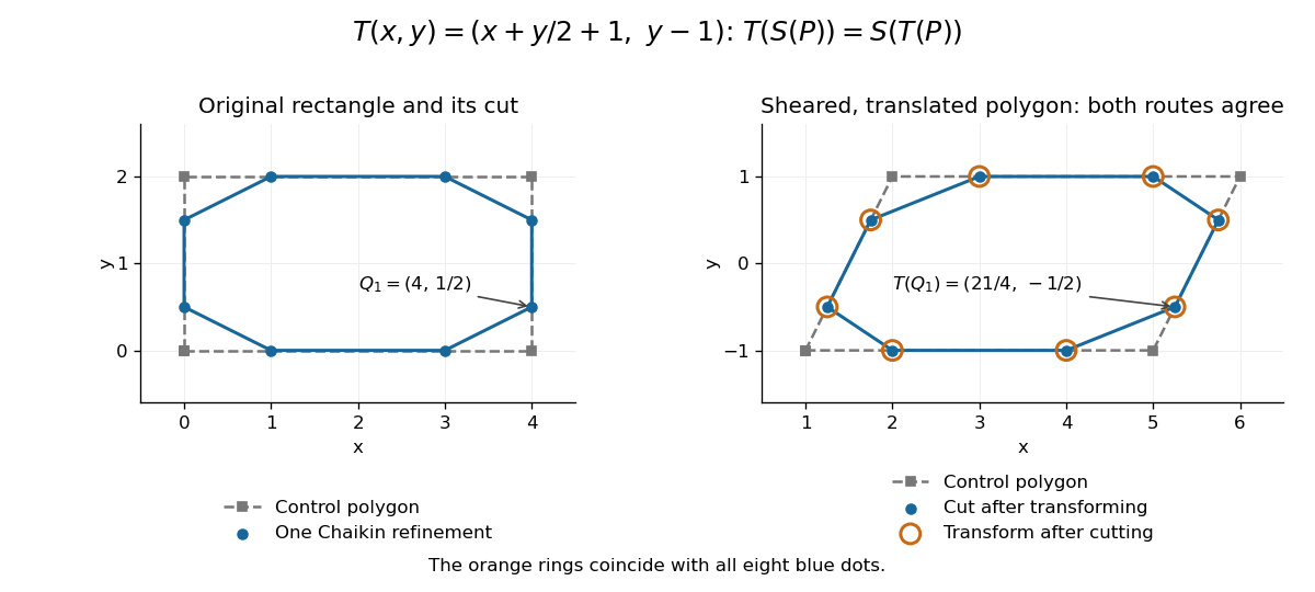
Shearing and translating a control polygon commutes with one Chaikin refinement
. Left: the rectangle and its first refinement. Right: the transformed control polygon, with blue dots from cutting after the affine map and orange rings from applying the affine map after cutting. All eight pairs coincide. Details.Historically, George M. Chaikin published “An algorithm for high-speed curve generation” in Computer Graphics and Image Processing 3(4), December 1974, pages 346–349. Its emphasis was practical curve generation through a recursive algorithm using simple arithmetic, with applications including machine control and three-dimensional curves. The lasting appeal of Chaikin subdivision is how an elementary local average creates an entire smooth B-spline curve.[ref]
https://doi.org/10.1016/0146-664X(74)90028-8. G. M. Chaikin, An algorithm for high-speed curve generation, Computer Graphics and Image Processing 3(4), 346–349, 1974; publisher metadata and abstract
The functional precision set of a subdivision scheme consists of functions exactly reproduced by refining their uniform samples with the scheme's consistent parameter placement. Polynomial precision usually specifies the reproduced polynomial space. If exactness is required for every grid spacing and shift, the binary midpoint-interpolation scheme has precision exactly the affine functions. At one fixed grid, its entire reconstruction range is the space of continuous piecewise linear functions on that grid; this larger range should not be confused with polynomial precision or arbitrary-grid reproduction.
The centered subdivision mask retains old control points and inserts edge midpoints. Its control polygon is unchanged as a geometric curve by refinement. Its basic limit is the hat , with support . This linear spline representation reproduces constants and linear functions, and is but generally not at its spline knots.
For a tripartite density operator ,Equivalently, conditioning on an additional quantum system cannot increase quantum conditional entropy.
Pinned article: Introduction to the OurBigBook Project
Welcome to the OurBigBook Project! Our goal is to create the perfect publishing platform for STEM subjects, and get university-level students to write the best free STEM tutorials ever.
Everyone is welcome to create an account and play with the site: ourbigbook.com/go/register. We belive that students themselves can write amazing tutorials, but teachers are welcome too. You can write about anything you want, it doesn't have to be STEM or even educational. Silly test content is very welcome and you won't be penalized in any way. Just keep it legal!
Intro to OurBigBook
. Source. We have two killer features:
- topics: topics group articles by different users with the same title, e.g. here is the topic for the "Fundamental Theorem of Calculus" ourbigbook.com/go/topic/fundamental-theorem-of-calculusArticles of different users are sorted by upvote within each article page. This feature is a bit like:
- a Wikipedia where each user can have their own version of each article
- a Q&A website like Stack Overflow, where multiple people can give their views on a given topic, and the best ones are sorted by upvote. Except you don't need to wait for someone to ask first, and any topic goes, no matter how narrow or broad
This feature makes it possible for readers to find better explanations of any topic created by other writers. And it allows writers to create an explanation in a place that readers might actually find it.
Figure 1. Screenshot of the "Derivative" topic page. View it live at: ourbigbook.com/go/topic/derivativeVideo 2. OurBigBook Web topics demo. Source. - local editing: you can store all your personal knowledge base content locally in a plaintext markup format that can be edited locally and published either:This way you can be sure that even if OurBigBook.com were to go down one day (which we have no plans to do as it is quite cheap to host!), your content will still be perfectly readable as a static site.
- to OurBigBook.com to get awesome multi-user features like topics and likes
- as HTML files to a static website, which you can host yourself for free on many external providers like GitHub Pages, and remain in full control

Figure 2. You can publish local OurBigBook lightweight markup files to either OurBigBook.com or as a static website.
Figure 3. Visual Studio Code extension installation.
Figure 5. . You can also edit articles on the Web editor without installing anything locally. Video 3. Edit locally and publish demo. Source. This shows editing OurBigBook Markup and publishing it using the Visual Studio Code extension. 
- Infinitely deep tables of contents:




All our software is open source and hosted at: github.com/ourbigbook/ourbigbook
Further documentation can be found at: docs.ourbigbook.com
Feel free to reach our to us for any help or suggestions: docs.ourbigbook.com/#contact