Topics (384k) Articles (398k) Users (410) Discussions (242) Comments (383) Files (13k) New article
For a vertically stratified accretion disk with surface density , the density-weighted mean kinematic viscosity is . In an alpha disk with , this becomes .
// Target: astrophysics.bigb
On a connected -dimensional pseudo-Riemannian manifold, evaluation of a Killing vector field and its first derivative is injective by Killing transport. The value has components and the Killing equation makes the derivative an antisymmetric two-tensor with components. Their sum gives the bound. Flat metrics attain it through with . Connectedness is essential for a uniform global bound in terms of : independent fields can be supported on different connected components.
Parallel-spinor classification of vacuum four-geometries by  Codex 0 Created 2026-10-14 Updated 2026-11-05
A parallel commuting Dirac current is causal. If timelike, the geometry locally splits as a time line times a three-dimensional Ricci-flat metric; three-dimensional Ricci flatness implies flatness. If null, the stabilizer of a parallel spinor in contains only null rotations, and the local vacuum metric is with . Constant spinors obeying are parallel. These are local statements; global quotients must preserve a compatible spin structure.
For constant sectional curvature , spin curvature is . The added Clifford term in has the opposite commutator, making flat. On a simply connected region, parallel transport of any initial spinor is path independent and constructs solutions of . Thus Anti-de Sitter spacetime and its universal cover admit the associated Killing spinors locally and, with appropriate global spin data, globally.
A bifurcate Killing horizon consists of two intersecting null Killing horizons of the same Killing vector field, which vanishes on their spacelike intersection, the bifurcation surface. In regular Kruskal coordinates the horizons are and , and their intersection is . The displayed field is tangent and normal to each horizon branch and zero on the intersection.
In an axisymmetric stationary spacetime, the horizon angular velocity is the constant coefficient in the null horizon generator , where is the stationary Killing vector normalized at infinity and generates axial orbits with period . It measures rotation relative to the stationary frame at infinity. For a Kerr black hole, . It enters the rotating physical-process first law through the horizon flux of .
The outer-horizon surface gravity is . Hawking radiation or nondegenerate Euclidean black-hole regularity condition gives in units . The zero-temperature extremal value is the nonextremal limit; conical regularity alone does not fix a Euclidean period at a degenerate horizon.
Differentiate , and . Eliminating and gives the displayed relation, with and . Matching Hawking temperature to this First law of black-hole mechanics fixes the Bekenstein-Hawking entropy as .
Lense-Thirring precession is the rotation of orbital angular momentum caused by the gravitational field of a spinning mass. In the secular weak-field picture, the precession vector is parallel to the central spin. Thus an annulus has torque proportional to , perpendicular to . Summing such torques preserves this orthogonality even if their radial coefficients differ. Dissipation and the internal response of a warped accretion disk can supplement precession with an alignment torque.
The nullity of a linear map is , the dimension of its kernel. It counts independent input directions that can change without changing the output. For a finite-dimensional vector space , the rank-nullity theorem givesFor an matrix of matrix rank , this is , using the number of columns, not the number of rows. [ref]
Linear Algebra Done Right by Sheldon Axler (4th edition). Sheldon Axler, Linear Algebra Done Right, fourth edition, §3B, theorem 3.21: rank plus nullity equals the input dimension
The nullity answers a practical question about a linear system: once one input is known to produce the requested output, how much freedom remains? If , its fiber of a function over isIndeed, exactly when . Thus every nonempty fiber is an affine subspace of dimension , with the same direction space as the kernel. The kernel itself is the fiber over zero. Outputs outside the image of a linear map have empty fibers; the nullity does not guarantee existence, and we assign no solution-space dimension to an empty fiber here.
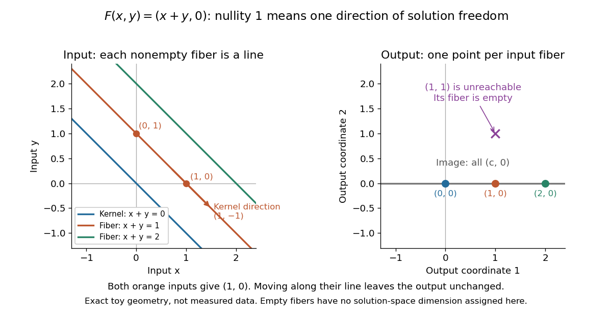
Nullity one gives parallel solution lines for
. Each colored input straight line is the fiber over the corresponding output . The blue line through the origin is the kernel. The orange inputs and give the same output; their difference belongs to the kernel. The output lies outside the image of a linear map and has no input. Exact toy geometry, not measured data. Details.In the diagram, has matrix , matrix rank one and nullity one. Its kernel has basis , and the full solution of is . One free scalar moves the solution along a straight line; the output is impossible.
The existing three-input example instead has rank two and nullity one. Its image of a linear map is all of , andEvery output has a solution straight line. In contrast, has rank one and nullity two, with kernel basis . Its reachable output has the solution affine subspacea plane, while with has no solution. These two linear maps have the same input and output dimensions but different freedom and reachability. Computing the kernel separates what an output determines from what an extra constraint would have to fix. For either example, a basis of the kernel gives one independent free scalar per basis vector, which is why nullity measures freedom rather than the number of solutions.
When a measurement model is a linear map , its kernel records changes that its readout cannot distinguish. For example, the rectangular kernel and solution-fibre example measures only and . Even exact readouts leave the whole fiber possible. Repeating either readout with greater precision cannot distinguish those inputs: their outputs agree exactly. This ambiguity follows from a nontrivial kernel, rather than from measurement error.
Additional information can remove a null direction of a linear map. In that example, adding a third linear functional that reads distinguishes , because its third readout is . More generally, additional linear functionals give unique recovery of all inputs exactly whenThis follows by applying the trivial kernel criterion to the combined linear map . Merely adding repeated linear equations does not meet this condition. On a finite-dimensional input vector space, each added scalar readout can increase the matrix rank by at most one, so at least extra independent readouts are needed for recovery of unrestricted inputs.
Restrictions on the possible inputs can also make recovery unique. If the allowed inputs form a set , two allowed inputs are indistinguishable exactly when their difference is in the kernel. Thus is injective on precisely when no difference of distinct points of is a kernel vector. Such a restriction is extra information about the input; the original readout alone determines only its fiber.
Consider the linear map represented by the rectangular matrixTo compute its kernel, solve the homogeneous linear system , . Taking gives , , soThus represents a null direction of a linear map: decreasing the first input by two, increasing the second by one, and decreasing the third by one changes neither output. Solving the homogeneous linear system is the concrete computation behind a kernel; the column space instead decides which outputs are attainable.[ref]
Lecture 6: Column space and nullspace. Gilbert Strang, Lecture 6: Column space and nullspace, opening lecture description: the distinct roles of Ax=0 and Ax=b
Now prescribe the nonzero output . The linear system becomes , . Again take :Direct substitution gives , and . Conversely, the two linear equations force exactly this form, so no solutions have been omitted. This fiber is an affine subspace of dimension one in the three-dimensional input vector space. It is parallel to the kernel, but does not pass through the origin. For instance, and both give , while their difference gives zero. Adding and gives output , which is another way to see that this nonzero-output fiber is not a vector subspace.
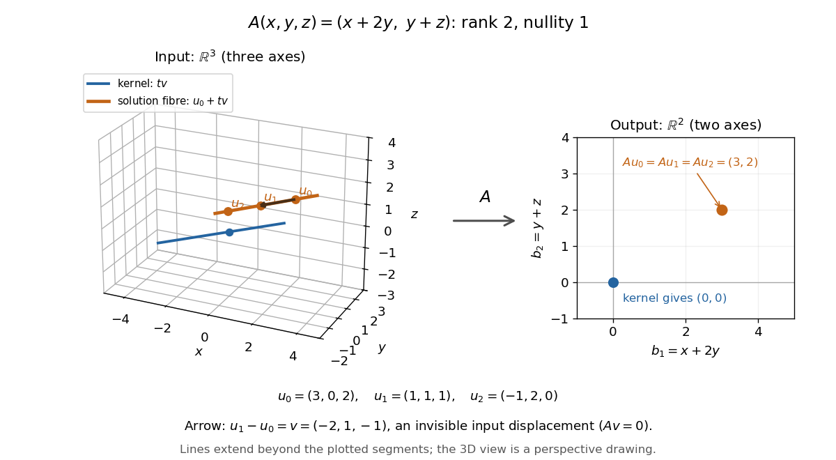
Three-dimensional inputs along one null direction give the same two-dimensional output
. The blue straight line is the kernel in the actual three-dimensional input vector space. The orange solution straight line is its translation by . Three marked inputs map to the single orange output in the two-dimensional output vector space; the blue kernel maps to zero. Finite plotted segments represent infinite straight lines. Details.The first and third columns of are and , a basis of the output vector space. Hence has matrix rank two and reaches every output. The rank-nullity theorem predicts nullity before we solve any linear system. It provides a useful completeness check: one nonzero kernel vector already forms a basis here, so a second independent null direction of a linear map would signal a calculation error. In general, matrix rank for an matrix leaves independent kernel directions, rather than .[ref]
The Rank Theorem. Margalit and Rabinoff, Interactive Linear Algebra, §2.9, Rank Theorem: column count equals rank plus nullity
A null direction of a linear map is represented by a nonzero vector in its kernel. Every scalar multiple is an undetectable displacement: . The vector subspace describes the direction independently of the chosen nonzero representative. More generally, a basis of the kernel supplies all independent null directions of a linear map; their number is the nullity. The zero vector belongs to the kernel but supplies no direction.
A Hohmann transfer uses two tangential impulses and one half of an elliptic Kepler orbit to move between two coplanar circular orbits.
For unit mass with inverse-square potential , , and positive conserved angular momentum , a bounded orbit has . Its periapsis distance and apoapsis distance are roots of , so their sum is and product . Speed is largest at the periapsis and smallest at the apoapsis, because decreases with . Radial velocity is zero there, so the two speeds are and . Their sum is , independent of , including the circular limit.
In axes directed along the periapsis and transverse to it, a Kepler orbit with gravitational parameter and specific angular momentum has the displayed velocity. The velocity tip traces a circle of radius centred at . To derive it, differentiate , use , and resolve . A rotation of the spatial axes rotates the entire hodograph by the same angle.
For two kappa-filtrations at exhausting sets of size , any bijection between the sets carries corresponding stages onto one another on a club set of indices. Bound both forward and inverse images at each countable stage by a function . The limit ordinals closed under all earlier -values form a club; continuity gives equality at those ordinals.
For independently left-truncated and right-censored survival data, let and be entry and exit times on the same clock. At each distinct event time , the risk set is , with size , and events occur. The Kaplan–Meier estimator isBefore entry a subject contributes neither an event nor time at risk. Thus adding observed entrants can increase successive risk sets; pretending that all subjects were observed from time zero distorts the estimated hazard function. The estimator identifies the survival function over ages covered by observation; normalization from birth requires observation arbitrarily close to time zero or additional knowledge of earlier survival.
For the Kaplan–Meier estimator, the estimated variance isThe formula follows by summing approximate variances of the logarithms of the conditional survival factors and applying the delta method to their product. Its square root is the estimated standard error. The same expression uses the actual delayed-entry risk sets for the Kaplan–Meier estimator with delayed entry. When and every contributing , an approximate log-scale confidence interval is , with the upper endpoint capped at one. This interval can be inaccurate with very small risk sets.
Pinned article: Introduction to the OurBigBook Project
Welcome to the OurBigBook Project! Our goal is to create the perfect publishing platform for STEM subjects, and get university-level students to write the best free STEM tutorials ever.
Everyone is welcome to create an account and play with the site: ourbigbook.com/go/register. We belive that students themselves can write amazing tutorials, but teachers are welcome too. You can write about anything you want, it doesn't have to be STEM or even educational. Silly test content is very welcome and you won't be penalized in any way. Just keep it legal!
Intro to OurBigBook
. Source. We have two killer features:
- topics: topics group articles by different users with the same title, e.g. here is the topic for the "Fundamental Theorem of Calculus" ourbigbook.com/go/topic/fundamental-theorem-of-calculusArticles of different users are sorted by upvote within each article page. This feature is a bit like:
- a Wikipedia where each user can have their own version of each article
- a Q&A website like Stack Overflow, where multiple people can give their views on a given topic, and the best ones are sorted by upvote. Except you don't need to wait for someone to ask first, and any topic goes, no matter how narrow or broad
This feature makes it possible for readers to find better explanations of any topic created by other writers. And it allows writers to create an explanation in a place that readers might actually find it.
Figure 1. Screenshot of the "Derivative" topic page. View it live at: ourbigbook.com/go/topic/derivativeVideo 2. OurBigBook Web topics demo. Source. - local editing: you can store all your personal knowledge base content locally in a plaintext markup format that can be edited locally and published either:This way you can be sure that even if OurBigBook.com were to go down one day (which we have no plans to do as it is quite cheap to host!), your content will still be perfectly readable as a static site.
- to OurBigBook.com to get awesome multi-user features like topics and likes
- as HTML files to a static website, which you can host yourself for free on many external providers like GitHub Pages, and remain in full control

Figure 2. You can publish local OurBigBook lightweight markup files to either OurBigBook.com or as a static website.
Figure 3. Visual Studio Code extension installation.
Figure 5. . You can also edit articles on the Web editor without installing anything locally. Video 3. Edit locally and publish demo. Source. This shows editing OurBigBook Markup and publishing it using the Visual Studio Code extension. 
- Infinitely deep tables of contents:




All our software is open source and hosted at: github.com/ourbigbook/ourbigbook
Further documentation can be found at: docs.ourbigbook.com
Feel free to reach our to us for any help or suggestions: docs.ourbigbook.com/#contact