For an integral generator $\alpha$ of a number field, let $A=\mathbb{Z}[\alpha ]$ and suppose $p$ is coprime to $[{\mathcal{O}}_K:A]$. Localizing at $p$ makes $A$ and the ring of integers equal, so reduction gives the displayed quotient ring. If $\overline{m}=\prod g_i^{e_i}$ with distinct monic irreducible polynomials, the Chinese remainder theorem gives local factors ${\mathbb{F}}_p[X]/(g_i^{e_i})$. Their residue fields have degrees $\mathrm{deg}{g}_i$ and their maximal ideals have nilpotence indices of an ideal $e_i$. Localizing the Dedekind domain ${\mathcal{O}}_K$ at the corresponding prime ideals gives discrete valuation rings, where this same nilpotence index of an ideal is the ramification index of a prime ideal. Thus $(p)=\prod (p,g_i(\alpha ){)}^{e_i}$ and each residue degree is $\mathrm{deg}{g}_i$.

For an algebraic integer $\alpha$ generating a number field, the polynomial discriminant of its minimal polynomial $f$ equals the discriminant of elements of a number field for its power basis. A squarefree reduction modulo $p$ has nonzero resultant with its derivative, so $p\nmid \mathrm{disc}(f)$. The discriminant-index formula for an integral lattice, $\mathrm{disc}(f)=[{\mathcal{O}}_K:\mathbb{Z}[\alpha ]{]}^2{d}_K$, proves the assertion.

// Target: arithmetic.bigb

For $d{s}^2=-fd{t}^2+d{r}^2/f+R^{2}d{\Omega }^2$, suppose $f$ and $R$ are analytic at $r_H$, $f(r_H)=0$, $f^{\prime }(r_H)=2\kappa >0$ and $R(r_H)>0$. The tortoise coordinate obeys the displayed expansion with analytic $h$. For $U=-e^{-\kappa (t-r_{\ast })}$ and $V=e^{\kappa (t+r_{\ast })}$ in the right exterior, $-UV=(r-r_H)e^{2\kappa h(r)}$ after fixing an additive constant. The inverse function theorem makes $r$ analytic in $UV$ through zero, while $d{s}^2=fdUdV/({\kappa }^{2}UV)+R^{2}d{\Omega }^2$ has a finite nonzero radial coefficient there. This supplies the local analytic extension and its bifurcate Killing horizon.

This radial spacetime diagram uses Kruskal–Szekeres coordinates to display both exteriors, the black hole and the white hole of maximally extended Schwarzschild spacetime. Each point represents a symmetry two-sphere. Radial null geodesics have slopes $\pm 1$ in the displayed coordinates; the horizons are $T_K=\pm X_K$ and the singularities satisfy $T_K^2-X_K^2=1$ in the usual normalization. A further compactification gives the corresponding Penrose diagram.

In Kruskal–Szekeres coordinates, every future-directed radial causal curve has nondecreasing $U$ and $V$. The right exterior has $U<0,V>0$, while the left has $U>0,V<0$. No future-directed causal curve can travel between the exteriors because it would have to decrease one null coordinate. The spatial bridge on a time-symmetric slice is therefore not a traversable passage.

For sufficiency, let $N$ be composite and squarefree, with $p-1\mid N-1$ for every prime factor $p$. For any integer $a$ coprime to $N$, Fermat's little theorem gives $a^{N-1}\equiv 1(\mathrm{mod}p)$ for every such $p$. Their product is $N$, so the Chinese remainder theorem gives the required congruence modulo $N$.

For necessity, first rule out a repeated factor. If $N=p^{k}m$ with $k\ge 2$ and $\gcd (p,m)=1$, the Chinese remainder theorem supplies $a\equiv 1+p(\mathrm{mod}{p}^k)$ and $a\equiv 1(\mathrm{mod}m)$. This $a$ is coprime to $N$. But the binomial theorem givescontradicting the Carmichael number condition. Hence $N$ is squarefree.

Now choose a primitive root $g$ modulo a prime factor $p$. Lift it to a unit modulo $N$ by prescribing $a\equiv g(\mathrm{mod}p)$ and $a\equiv 1(\mathrm{mod}N/p)$. The Chinese remainder theorem applies because $N$ is squarefree. The Carmichael congruence implies $g^{N-1}\equiv 1(\mathrm{mod}p)$. Since $g$ has multiplicative order $p-1$, that order divides $N-1$. This proves the other condition.^[ref]

For positive linear operators on continuous functions on $[0,1]$, put $e_j=U_n(x^j)-x^j$. Uniform continuity supplies the barriers $|f(x)-f(t)|\le \epsilon +\gamma (x-t{)}^2$. Applying positivity and evaluating at $t$ gives the displayed estimate because $U_n((x-t{)}^2)(t)=e_2(t)-2t{e}_1(t)+t^2{e}_0(t)$. The constant $\gamma$ is independent of $t$ and $n$. Thus uniform reproduction of $1,x,x^2$ proves Korovkin theorem convergence on every continuous function; exact reproduction forces the operator to be the identity.

The Compton y parameter is the Thomson scattering optical depth weighted by the dimensionless electron temperature. It measures the integrated electron pressure along a line of sight. When hot, nonrelativistic electrons scatter much colder photons, the first-order radiation energy gain is $4y$ times the incident energy. The spectrum is redistributed while the total photon number density is conserved locally by scattering.

The two-sample Kolmogorov-Smirnov test compares two empirical distribution functions from independent samples, each internally independent and identically distributed, under the null hypothesis that their underlying probability distributions coincide. Both curves are estimated from data, so calibration depends on both sample sizes; the usual asymptotic scaling is $\sqrt{nm/(n+m)}{D}_{n,m}$. Tied data can be handled by an appropriate permutation test under the required exchangeability, rather than by assuming the untied continuous-null law.^[ref]

The Lilliefors test calibrates the Kolmogorov-Smirnov statistic against a normal distribution whose mean and variance are estimated from the tested observations. In the original procedure, $s^2$ is the sample variance with denominator $n-1$, and $\Phi$ is the standard normal distribution function. Its reference law includes this fitting step. The original paper's opening procedure and Table 1 explain the changed calibration.^[ref]

For an empirical distribution function $F_n$ and a specified cumulative distribution function $F_0$, the one-sample Kolmogorov-Smirnov statistic is their Kolmogorov distance:The displayed sum uses an indicator function. With this convention, $F_n$ is right-continuous. For distinct observations, its value and its left one-sided limit at the $i$th order statistic are $F_n(X_{(i)})=i/n$ and $F_n(X_{(i)}^{-})=(i-1)/n$.

For continuous $F_0$, both jump sides matter. Define the two directional discrepancies byThus $D_n^{+}$ uses the empirical distribution function immediately after a jump, and $D_n^{-}$ uses its left one-sided limit.^[ref] A supremum need not be attained.

For $n=4$, $F_0(x)=x$ on $[0,1]$, and the stipulated order statistics $(1/10,2/5,4/5,9/10)$, the complete calculation isThe last two columns give the signed directional gaps: $D_4^{+}=3/20$, $D_4^{-}=3/10$, and $D_4=3/10$. In contrast, checking only $|F_4(X_{(i)})-F_0(X_{(i)})|$ gives $3/20$ and misses the largest gap approached as $x\uparrow 4/5$. At $x=4/5$ itself, the gap has already fallen to $1/20$.

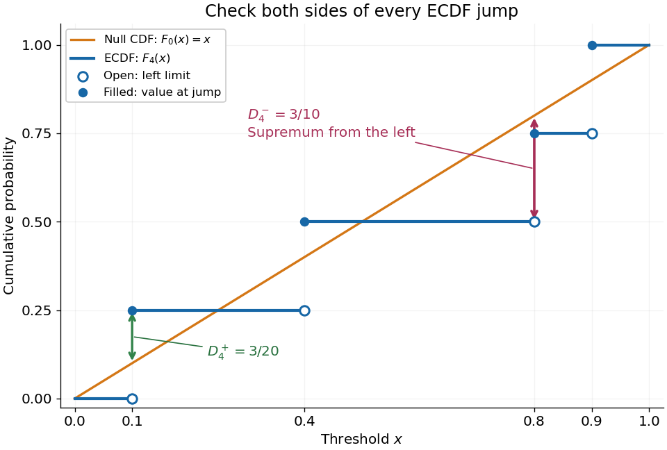
The finite formula follows from the behavior between jumps: the empirical distribution function $F_n$ is constant and the cumulative distribution function $F_0$ is monotone, so the largest directional gaps occur at the two interval ends, possibly as one-sided limits. The two tails introduce no larger gap. Checking every jump side therefore gives the exact supremum.

A common normalized Kolmogorov-Smirnov statistic is $\sqrt{n}{D}_n$, which equals $3/5$ in this example. Its large-sample reference law comes from the Kolmogorov-Smirnov theorem. The unscaled $D_n$ remains the largest difference of cumulative probabilities, not a p-value.

There is a useful exact exception to the usual warning about fitting statistical parameters. Suppose $n\ge 2$ independent and identically distributed observations have the uniform distribution on $(0,\theta )$ with unknown $\theta >0$. Let $M={\max }_i{X}_i$ and let $J$ be the label of its almost surely unique maximizing observation. Conditional on $M=m$ and $J=j$, the surviving labelled observations $(X_i{)}_{i\ne j}$ are independent with the uniform distribution on $(0,m)$; after division by $m$ they are independent and identically distributed uniforms on $(0,1)$. These are conditional distributions defined by probability density functions, since the event $M=m$ has probability zero.

To check this, the joint probability density function of $M$ and $J=j$ is $m^{n-1}/{\theta }^n$ for $0<m<\theta$. Dividing the original joint probability density function ${\theta }^{-n}$ by this factor gives the conditional survivor probability density functionThis factorization proves the claimed conditional independence; scaling removes $m$. Keep the surviving labels in a fixed order, or apply an independent random permutation. The sorted survivors instead have the joint law of uniform order statistics and exhibit statistical dependence; sorting does not affect their empirical distribution function. Delete the maximum itself, which would otherwise become a forced value $1$, and compute the Kolmogorov-Smirnov statistic using sample size $n-1$ and jump heights $i/(n-1)$. This gives an exact conditional Kolmogorov-Smirnov test under the uniform-endpoint statistical model. It does not justify fitting an arbitrary endpoint or other statistical parameters and using the ordinary $n$-sample calibration.

For five pairs of continuous functions on $[0,1]$, one can arrange that at every arbitrarily fine scale there are closed interval families whose product rectangles cover each point at least three times, and within each family the images under $a_q(x)+b_q(y)$ are mutually disjoint. To see this, put gaps near five shifted fine grids; gap sets for different shifts are disjoint. Each coordinate misses at most one family, so a pair misses at most two. Approximate any prescribed pair of functions by constants on the complementary intervals, interpolating across gaps. Perturb the finitely many constants to avoid all equalities between distinct pair sums. The rectangle images are then separated by a positive distance, a property preserved under sufficiently small uniform perturbations. For each required mesh size this property defines a dense open subset of $C([0,1]{)}^{10}$. The Baire category theorem gives a tuple satisfying every scale simultaneously.

For $f\in C({\mathbb{R}}^2)$, choose a positive continuous function $A$ with $A(t)\ge (1+t){\max }_{x^2+y^2\le t}|f(x,y)|$ for $t\ge 0$. Such an $A$ is obtained by piecewise linear interpolation of a sufficiently large increasing sequence. Then $b(x,y)=f(x,y)/A(x^2+y^2)$ tends uniformly to zero at infinity. Transport $b$ to $(0,1{)}^2$ by $x=\tan (\pi (s-1/2))$ and extend it by zero on the boundary; the extension is continuous. Apply the compact Kolmogorov-Arnold representation theorem, then multiply by $A(x^2+y^2)$. Multiplication introduces no additional primitive operation because $uv=[(u+v{)}^2-(u-v{)}^2]/4$ uses only addition and continuous one-variable squaring and scaling.

Under $z\mapsto (az+b)/(cz+d)$ with $ad-bc=1$, the coordinate measure contributes $|c{z}_i+d{|}^{-4}$ at insertion $i$. The Koba-Nielsen factor contributes $|c{z}_i+d{|}^{-{\alpha }^{\prime }{\sum }_{j\ne i}{p}_i\cdot p_j}$. Four-momentum conservation makes this exponent ${\alpha }^{\prime }{p}_i^2$, so the factors cancel precisely on the displayed tachyon mass shell. The correlator alone is covariant; its product with all the coordinate measures is invariant.

For $\mathrm{Kn}\ll 1$, frequent gas–gas collisions can establish a local Maxwellian before macroscopic conditions change appreciably. Under this additional near-equilibrium assumption, the hydrodynamic limit of the Boltzmann equation motivates a continuum approximation with Navier-Stokes equations and heat conduction. A no-slip boundary condition is a leading wall approximation, not a statement about individual molecular velocities.

With a small but finite Knudsen number, a useful slip approximation retains continuum bulk equations and corrects wall velocity and temperature. A Navier slip boundary condition can represent the leading tangential velocity correction, but its slip length must come from the relevant gas–wall interaction model. A nearby Knudsen layer still requires kinetic treatment if its detailed structure is wanted. Slip corrections are perturbations; extending them into order-one Knudsen numbers has no general accuracy guarantee. At order-one Knudsen number, wall and intermolecular collisions both matter; this transitional situation calls for a kinetic theory model. At $\mathrm{Kn}\gg 1$, free molecular flow becomes a useful limiting approximation. These are scale comparisons, with accuracy depending on geometry, flow conditions and the observable, rather than universal sharp numerical boundaries. ^[ref]

Suppose a known list of $2^m$ distinct $n$-bit strings $a_j$ is available and computational basis transpositions on $n+m$ qubits have polynomial-size implementations. Start with the uniform superposition state of index labels $j$, leaving the data zero. First swap $|0^n,j⟩$ with $|a_j,j⟩$ for each nonzero $a_j$. Next, for each $j\ne 0$, swap $|a_j,j⟩$ with $|a_j,0^m⟩$. Distinct index labels separate the first-stage pairs, and distinct data strings separate the second-stage pairs. Thus no later transposition disturbs an earlier term. At most $2^{m+1}-1$ transpositions prepare the uniform data state and return the quantum ancilla to zero. For $m=O(\log n)$ the quantum circuit has polynomial size. This assumes the list is available; a membership predicate alone does not supply it.

An alternating knot is a knot admitting an alternating knot diagram. A nonalternating diagram can still represent an alternating knot; the property of the knot is existential over its diagrams.

The matrix $C$ in the Knill--Laflamme condition is positive semidefinite, since $v^{†}Cv$ is the squared norm of ${\sum }_a{v}_a{E}_a|\psi ⟩$ for any normalized code state. Diagonalizing it gives linear combinations $F_j$ with $P{F}_j^{†}{F}_{l}P=c_j{\delta }_{jl}P$. For $c_j>0$, $V_j=F_{j}P/\sqrt{c_j}$ is an isometry of the code into an error-image subspace, and these subspaces are orthogonal. Measuring their projectors and applying $V_j^{†}$ recovers the logical state. Complete the operation arbitrarily on the orthogonal complement to obtain a quantum channel. This construction corrects every noise map whose Kraus operators lie in the specified error span, including coherent superpositions of error operators.

If a common recovery quantum channel with Kraus operators $R_{\mu }$ restores every pure code state after each error $E_a$, then each vector $R_{\mu }{E}_a|\psi ⟩$ is parallel to $|\psi ⟩$. Linearity on basis vectors and their pairwise superpositions forces $R_{\mu }{E}_{a}P=c_{\mu a}P$, with the scalar independent of the logical state. Insert ${\sum }_{\mu }{R}_{\mu }^{†}{R}_{\mu }=I$ between two error operators to obtain the displayed Knill--Laflamme condition. This proves necessity without presuming an orthogonal syndrome description of recovery.

For a free real scalar field expanded with measure $d^{3}p/[(2\pi {)}^{3}2E_p]$ and $f_p=e^{-ip\cdot x}$, the displayed Klein-Gordon inner product extracts its annihilation operator. Indeed $(f_p,f_q)=(2\pi {)}^{3}2E_p{\delta }^3(\mathbf{p}-\mathbf{q})$ and $(f_p,f_q^{\ast })=0$; spatial Fourier inversion removes the measure. Taking the Hermitian adjoint gives $a^{†}(\mathbf{p})=-i\int d^{3}x{f}_p\overleftrightarrow{{\partial }_t}\varphi$. The equal-time canonical commutation relation then gives $[a(\mathbf{p}),a^{†}(\mathbf{q})]=(2\pi {)}^{3}2E_p{\delta }^3(\mathbf{p}-\mathbf{q})$.