Topics (384k) Articles (398k) Users (410) Discussions (242) Comments (383) Files (13k) New article

A genuinely closed steady channel with impermeable sidewalls and ends must have zero integrated axial cell flux through every section, not only zero fluid flux. In the bulk phototactic ansatz , , and , the axial flux is . Meanwhile the momentum equation, zero fluid flux and integration by parts give . Thus a nontrivial bulk profile is generally incompatible with exact closed-end cell conservation unless the prefactor vanishes. Additional axial concentration variation is needed; neglecting end regions does not itself remove this global constraint.
For , a Prüfer sequence is the encoding of a labelled tree on by a sequenceRepeated labels are allowed, and their order matters. To encode the tree, repeatedly remove its smallest-labelled leaf of a graph together with its incident edge, recording the label of its unique neighbour. Stop when two vertices remain; do not record their final edge. Removing a leaf of a graph leaves a tree, so the procedure makes exactly deletions. The choice of the smallest label makes the encoding deterministic. [ref]
https://users.math.msu.edu/users/magyarp/math481/. Peter Magyar, Math 481: Prüfer encoding with the smallest leaf
For a concrete example, take six vertices and the set of edgesInitially label the vertices of vertex degree one. Remove and record its neighbour . Now has become a leaf of a graph, so remove and record . Next remove and record again; then remove and record . The final edge joins and . Thus the Prüfer sequence isThe deletion order is : removing a leaf of a graph can make its neighbour a leaf of a graph, so the eligible labels change as the tree shrinks.
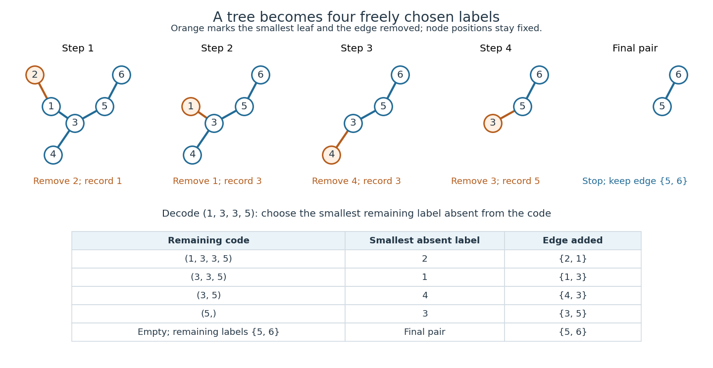
To decode, keep a set of remaining labels, initially , and the remaining sequence, initially . While the sequence is nonempty, let be the smallest label in absent from the entire remaining sequence. Add an edge between and its first entry, then remove from and delete that first entry. Finally join the two labels left in . For the example:
The decoder always has a choice: if the remaining sequence has length , then has labels, so at least two of them are absent. Its first entry is still in , and differs from the chosen absent label. Every removed vertex attaches to a vertex that survives longer; following these attachments eventually reaches the final pair. Consequently the decoded graph is connected, and its edges make it a tree. In this construction, each occurrence of contributes an incident edge, and gets one more edge at its final attachment. Thus a remaining label is absent from the remaining sequence exactly when it labels a leaf of a graph. Encoding and decoding choose the same smallest label at each step and undo each other. This bijection proves Cayley's formula and explains why every freely chosen sequence is valid. [ref]
https://www.cs.columbia.edu/~cs4203/files/GT-Lec4.pdf. Columbia University, Graph Theory Lecture 4: Prüfer degree identity, decoding algorithm, and bijection
For there is exactly one empty sequence, and decoding adds the sole edge. For there is one tree, with vertex degree zero, but no length- Prüfer sequence. This is the exception both to the encoding convention and to the Prüfer degree formula.
Heinz Prüfer's 1918 paper "Neuer Beweis eines Satzes über Permutationen" appeared in Archiv der Mathematik und Physik, third series, volume 27, pages 142–144. It gives an encoding proof of the labelled tree count. The historical title means "New proof of a theorem on permutations"; the modern Prüfer sequence permits repeated labels, so it is not a permutation. [ref]
https://i.sstatic.net/WDvxyMwX.png. Prüfer (1918), original opening-page scan, page 142
For a fixed set of roots among labelled vertices, the number of forests with exactly one root in each graph component is . Orient edges toward their roots. Repeatedly remove the smallest nonroot leaf and record its parent. This gives a code of length whose last entry is a root. Conversely, for any such code choose the smallest remaining nonroot absent from the remaining code, join it to the first entry, and delete it. There is always a choice because the final entry is a root. These inverse operations give choices for the earlier entries and for the last. For , the empty forest is unique.
For the additive infinite cyclic group , the generating set of a group produces the infinite line: each integer is adjacent to and . Adding the moves gives and additional edges skipping one vertex. Each skip still costs one step in the word metric.
For integers , these word metrics areThe absolute value counts unit moves, and the ceiling function counts pairs plus a possible leftover unit. Every -move changes the integer by at most two, while moves of size two followed by at most one move of size one attain this bound. For example, the graph path has five steps for , while has three for . This calculation gives the concrete comparison
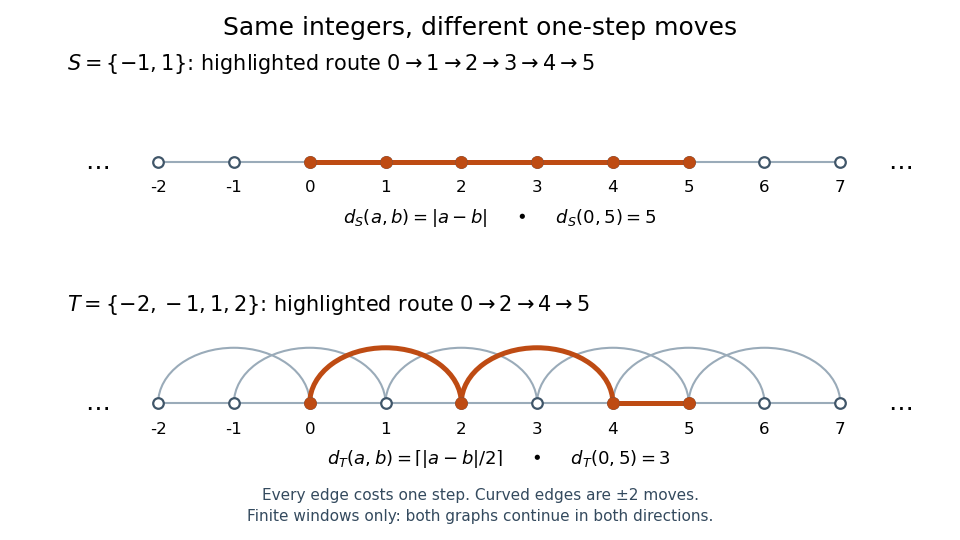
Two Cayley graphs of the integers: unit moves need five steps from zero to five; adding moves of size two needs three
. Details. The picture shows only a finite window of each infinite Cayley graph. By contrast, alone fails to be a generating set of a group for : it generates the subgroup . Its move graph has two connected components of a graph, the even integers and the odd integers. Within either component the graph distance is ; between different components no finite graph path exists. Adding a shortcut is different from deleting the moves needed for connectivity.
For with data along , the initial curve is noncharacteristic when its tangent is linearly independent of the projected characteristic vector evaluated at the initial value of . The determinant is , up to sign. For coefficients and data this permits the inverse function theorem to invert the local characteristic parametrization and gives a unique local classical solution.
Choose distinct and weights at spectral points . With and , solve . The reconstructed multisoliton solution is . Since , cyclicity of the trace gives . The Cauchy matrix is positive definite, because it is the Gram matrix of on ; diagonal similarity then proves . For one spectral point this yields .
Apply the symmetric-function involution in one alphabet to the ordinary Cauchy identity. It changes complete generators to elementary ones and, by the dual Jacobi–Trudi identity, sends to . This proves the identity as a formal series and relates pairings with transposed Young shapes to squarefree matrix weights.
Given with , put for . The Cauchy identity for symmetric functions and Jacobi–Trudi identity give , degree by degree in the completion. For the coefficients are ; for they are .
For a holomorphic function on a neighbourhood of a closed disc, parametrize the Cauchy derivative formula on its boundary. The conjugate Cauchy integral theorem gives . Replacing in the derivative integral by therefore gives the displayed identity. The boundary real part determines every nonconstant analytic coefficient; only an imaginary additive constant is lost.
A compact object (mathematics) is an object whose represented Hom functor preserves filtered colimits. This preservation condition differs from the extra right-adjoint property defining a tiny object.
An object is projective when every morphism lifts through every epimorphism . Equivalently, the functor preserves epimorphisms.
An object with the displayed property is called small projective; the term 0-presentable here uses this all-small-colimits convention. In a presheaf category, every representable presheaf has this property by the Yoneda lemma and pointwise computation of colimits. Conversely the canonical colimit presentation of a presheaf shows that the identity on such an object factors through one representable, making it a retract. If the indexing category has equalizers, a representable retract is again representable by the representable retract criterion.
A categorical morphism is an arrow with a specified source and target in a category. An arrow composes with to give . Composition is associative, and every object has an identity arrow acting as a unit. A functor preserves the sources, targets, identities and compositions of these arrows. In a locally small category, the arrows between fixed objects form a hom-set.
Reversing the arrows in a categorical statement produces its dual statement. A theorem holding for all categories therefore has a dual theorem obtained by applying it to the opposite category; for example, categorical limits are exchanged with colimits.
Transition state theory relates an elementary reaction's rate constant to a Gibbs energy of activation. The Eyring expression used in the catalyst example assumes every passage counted at the transition state succeeds. More generally, a factor accounting for unsuccessful passage multiplies it. Comparing barriers alone gives the quoted speedup only when the remaining prefactors agree. Free-energy profiles can depend on temperature, so the example's values at do not determine a temperature curve. See the IUPAC Gold Book: transition state theory.
A Hadamard space is a complete CAT(0) space. Equivalently, it is a complete metric space in which every pair has a midpoint satisfyingfor every . A midpoint means . Substituting a second midpoint for forces their distance to be zero, so the midpoint is unique.
Iterating midpoints defines the joining geodesic first at dyadic parameters. Completeness then supplies its points at every real parameter. The midpoint inequality extends by this approximation to the Hadamard squared-distance inequality, and hence to Euclidean triangle comparison. In particular, closed balls have geodesic convexity.
The completeness condition belongs in both formulations. The rational numbers with the usual distance have all rational midpoints and satisfy the displayed inequality, but are incomplete. A full real-parameter geodesic from zero to one would require irrational points. Thus the midpoint inequality alone does not make that space a Hadamard space.
For an integral domain with fraction field , realize Cartier divisors as invertible fractional ideals, with local divisor equation corresponding to the ideal . This is the convention. The maps in the displayed exact sequence are unit inclusion, , and . A principal fractional ideal is trivial as a divisor exactly when its generator is a unit. An invertible fractional ideal is trivial in the Picard group of a ring exactly when it is principal. Every rank-one projective module embeds in and produces an invertible fractional ideal, proving surjectivity. Local multiplication identifies with , so these are group homomorphisms.
For a morphism of varieties , pull back local defining rational functions of a Cartier divisor whenever they remain nonzero on each component of . Their ratios remain regular units, defining . Equivalently, pull back the associated line bundle and its rational section. A dominant morphism always permits this construction.
Pinned article: Introduction to the OurBigBook Project
Welcome to the OurBigBook Project! Our goal is to create the perfect publishing platform for STEM subjects, and get university-level students to write the best free STEM tutorials ever.
Everyone is welcome to create an account and play with the site: ourbigbook.com/go/register. We belive that students themselves can write amazing tutorials, but teachers are welcome too. You can write about anything you want, it doesn't have to be STEM or even educational. Silly test content is very welcome and you won't be penalized in any way. Just keep it legal!
Intro to OurBigBook
. Source. We have two killer features:
- topics: topics group articles by different users with the same title, e.g. here is the topic for the "Fundamental Theorem of Calculus" ourbigbook.com/go/topic/fundamental-theorem-of-calculusArticles of different users are sorted by upvote within each article page. This feature is a bit like:
- a Wikipedia where each user can have their own version of each article
- a Q&A website like Stack Overflow, where multiple people can give their views on a given topic, and the best ones are sorted by upvote. Except you don't need to wait for someone to ask first, and any topic goes, no matter how narrow or broad
This feature makes it possible for readers to find better explanations of any topic created by other writers. And it allows writers to create an explanation in a place that readers might actually find it.
Figure 1. Screenshot of the "Derivative" topic page. View it live at: ourbigbook.com/go/topic/derivativeVideo 2. OurBigBook Web topics demo. Source. - local editing: you can store all your personal knowledge base content locally in a plaintext markup format that can be edited locally and published either:This way you can be sure that even if OurBigBook.com were to go down one day (which we have no plans to do as it is quite cheap to host!), your content will still be perfectly readable as a static site.
- to OurBigBook.com to get awesome multi-user features like topics and likes
- as HTML files to a static website, which you can host yourself for free on many external providers like GitHub Pages, and remain in full control

Figure 2. You can publish local OurBigBook lightweight markup files to either OurBigBook.com or as a static website.
Figure 3. Visual Studio Code extension installation.
Figure 5. . You can also edit articles on the Web editor without installing anything locally. Video 3. Edit locally and publish demo. Source. This shows editing OurBigBook Markup and publishing it using the Visual Studio Code extension. 
- Infinitely deep tables of contents:




All our software is open source and hosted at: github.com/ourbigbook/ourbigbook
Further documentation can be found at: docs.ourbigbook.com
Feel free to reach our to us for any help or suggestions: docs.ourbigbook.com/#contact