Topics (384k) Articles (398k) Users (410) Discussions (242) Comments (383) Files (13k) New article

A clipped waveform area is the integral of an amplitude-limited trace over the specified interval. It can differ from the unclipped area by a different proportion than the change in peak height. The amplifier clipping article gives the instantaneous limiter model and a rectangular-pulse example; real saturated integrators can also have recovery dynamics.[ref]
ACF2101 Low Noise, Dual Switched Integrator datasheet. p10, Output Overload
An original triangular example takes with . Its true area is . Clip its top at , with the zero baseline unchanged. The missing region is a triangle of height and base , soFor , and , the area falls from to . The peak is halved but the area loses only . The clipping loss for a triangular pulse therefore cannot be inferred merely by applying the peak-loss percentage to its integral.
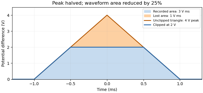
Record input and output together while changing gain or attenuation to test whether the trace is clipped. Recovering area by fitting an assumed triangle is a model-based correction, not recovery of an arbitrary waveform from its plateau. Baseline errors, limited bandwidth and overload recovery require their own measurement models.
Glucosamine is an amino sugar, conventionally 2-amino-2-deoxy-D-glucose. Relative to the open-chain glucose reference structure, its carbon-2 hydroxy group is replaced by an amino group, with the corresponding stereochemical arrangement retained.[ref]
Nomenclature of Carbohydrates (Recommendations 1996) by Alan D. McNaught. Section 2-Carb-14: D-glucosamine and amino-deoxy naming
Replacing by removes one oxygen and adds one nitrogen and one hydrogen. Thus the neutral free base has molecular formula , compared with for glucose. This is structural bookkeeping, not a claim that every preparation is made by one replacement reaction.
N-acetylglucosamine further modifies that nitrogen. Distinguishing the two names matters when identifying a polysaccharide's building blocks: an acetyl group changes chemical identity even though the six-carbon framework remains recognizable.[ref]
Nomenclature of Carbohydrates (Recommendations 1996) by Alan D. McNaught. Section 2-Carb-25: amino-sugar nitrogen substitution
N-acetylglucosamine is the N-acetyl derivative of glucosamine, commonly the D sugar. Its carbon-2 nitrogen carries an acetyl group, forming an amide; the open-chain reference name is 2-acetamido-2-deoxy-D-glucose.[ref]
Nomenclature of Carbohydrates (Recommendations 1996) by Alan D. McNaught. Sections 2-Carb-14 and 2-Carb-25: amino-deoxy naming and N-substitution
Compare with . Replacing one nitrogen-bound hydrogen by an acetyl group changes the atom inventory by , giving neutral molecular formula . The nitrogen remains part of the amino sugar derivative even though it is no longer a free amino group.
Hyaluronic acid alternates N-acetylglucosamine with glucuronic acid. In the hyaluronan synthase experiment of P. L. DeAngelis, the activated donor UDP-N-acetylglucosamine provided this sugar type. An ideal segment with 20 complete two-sugar repeats contains 20 residues of each type and 40 sugar residues altogether.[ref]
Enzymological characterization of the Pasteurella multocida hyaluronic acid synthase by P. L. DeAngelis. Abstract: alternating composition and two activated sugar donors
N-acetylgalactosamine is an amino sugar derivative whose carbon2 nitrogen carries an acetyl group. In biological contexts the D sugar is usual; the systematic framework is 2-acetamido-2-deoxygalactose. The neutral free sugar has molecular formula . A broad name and a specific beta-D anomer are different levels of chemical specification.[ref]
An original atom-counting exercise starts with galactose, . Replacing its carbon2 by gives galactosamine, . Replacing one nitrogen-bound hydrogen with an acetyl group adds overall, producing . This is structural bookkeeping, not a proposed one-step laboratory synthesis.[ref]
Nomenclature of Carbohydrates (Recommendations 1996) by Alan D. McNaught. Sections2-Carb-14 and2-Carb-25: amino-deoxy sugars and nitrogen substitution
N-acetylgalactosamine and N-acetylglucosamine differ in carbon4 configuration. That epimerization is separate from changing anomeric configuration or adding/removing the acetyl group. A common formula alone cannot identify which arrangement is present.
In dermatan sulfate, residues of N-acetylgalactosamine form part of the linked sugar chain. A linked residue, the free monomer and an activated nucleotide-sugar donor should not be assigned the same complete molecular formula merely because they share this sugar name.[ref]
Galactosamine is an amino sugar derived from galactose by replacing its carbon-2 hydroxy group with an amino group. The conventional D compound is 2-amino-2-deoxy-D-galactose. Specifying the D configuration does not by itself specify the alpha or beta anomer of a cyclic form.[ref]
Nomenclature of Carbohydrates (Recommendations 1996) by Alan D. McNaught. Section 2-Carb-14: amino-sugar definition and accepted D-galactosamine name
The neutral free sugar has molecular formula . As an original atom-counting exercise, begin with galactose, . Replacing by removes one oxygen and adds one nitrogen and one hydrogen overall. This gives the stated formula; it is structural bookkeeping, not a claim that this substitution is a one-step laboratory synthesis.[ref]
D-galactosamine pyranose in ChEBI. CHEBI:60312, formula and pyranose identity; CHEBI:148869, explicitly alpha form
Galactosamine and glucosamine differ in the configuration at carbon4 of their corresponding D-sugar frameworks. Adding an acetyl group to the nitrogen instead produces N-acetylgalactosamine, a different structural modification. Neither relationship is determined by a formula alone: epimers can share a formula, while nitrogen substitution can change it.
In chondroitin, the chain contains N-acetylgalactosamine-derived residues rather than simply a collection of free galactosamine molecules. Distinguishing the free sugar, its nitrogen-modified derivative and its residue within a polysaccharide prevents confusing composition with molecular identity.
AC power describes energy transfer associated with time-varying electric potential difference and electric current, including the distinction between instantaneous transfer and its average. With the passive sign convention, current enters the terminal marked positive, and instantaneous power absorbed by the element is . A positive value means energy entering the element; a negative value means energy returning through that terminal pair.
For sinusoidal steady operation, choosewhere and are root mean square magnitudes. The cosine-product identity givesAveraging over a complete period removes the second term, giving active power . This derivation separates the energy-transfer average from a twice-frequency oscillation.[ref]
University Physics Volume 2 by Samuel J. Ling and others. §15.4, equations15.12–15.13, sinusoidal average power and RMS quantities
For an original example, , and give active power480W. The oscillating term has amplitude600W, so instantaneous power ranges from−120 to1080W. Over ten complete cycles at50Hz, the net energy absorbed is . Temporary negative power can accompany positive net transfer when an element stores and returns energy.
The product in volt-amperes is the apparent power. In the single-frequency sinusoidal convention, reactive power is , giving360 in reactive volt-amperes for a lagging current with . Complex electrical power packages and , while the power factor distinguishes net transfer from the terminal magnitude product. The primary MIT treatment derives these quantities and makes the peak-versus-RMS convention explicit.[ref]
AC Power Flow in Linear Networks by James L. Kirtley Jr.. Energy and Power, equations61–63; §7.1 RMS Amplitude
A measurement must retain the relative phase of the two channels. Multiplying separately measured RMS magnitudes gives apparent power, not generally active power. For nonsinusoidal signals, the time average of remains the definition of active power, but one phase angle need not describe every harmonic contribution.
RRR-alpha-tocopherol is the alpha-tocopherol configuration . The nomenclature identifies it with the naturally occurring stereoisomer described in the recommendations.[ref]
Nomenclature of Tocopherols and Related Compounds by IUPAC-IUB Joint Commission on Biochemical Nomenclature. Recommendations 11 and 12a; Table 1, entry 1
The prefix records three configurations; “alpha” separately identifies ring methyl substitution.R and S are descriptors assigned by stereochemical sequence rules. They do not by themselves specify the sign or magnitude of measured optical rotation. For this molecular structure, inverting all three stereocenters gives SSS, its enantiomer. Inverting only the ring center gives SRR, a diastereomer. Thus a change at one center is not the same operation as taking a mirror image of the whole molecule.
An original dilution example begins with 4.00 mg of pure RRR-alpha-tocopherol. If material is transferred quantitatively to a final volume of 25.00 mL, its mass concentration is . Using the alpha-tocopherol molar mass , its amount concentration is approximately .[ref] Identity, purity and final volume are independent inputs to that calculation.
By contrast, 4.00 mg of a stipulated equal eight-form all-rac-alpha-tocopherol mixture contains only 0.500 mg of the RRR configuration. Both samples have the same total alpha-tocopherol mass, but different stereoisomer composition. This is a chemical accounting comparison; it does not assign nutritional equivalence or a treatment effect.
A measurement intended to certify the RRR amount must distinguish stereochemistry, rather than reporting only the shared molecular formula. Appropriate standards and a selective analytical method determine what the stated purity actually means.
All-rac-alpha-tocopherol designates an alpha-tocopherol stereoisomer mixture containing all four pairs of enantiomers. The nomenclature does not require exactly equal proportions of the pairs.[ref]
Nomenclature of Tocopherols and Related Compounds by IUPAC-IUB Joint Commission on Biochemical Nomenclature. Recommendation 12e and Table 1, entry 4
It is a description of stereochemistry, rather than a different alpha ring-methylation pattern.The three stereocenters at , and permit the configurations RRR, RRS, RSR, RSS, SRR, SRS, SSR and SSS, with the letters read in that order. The enantiomer pairs are RRR/SSS, RRS/SSR, RSR/SRS and RSS/SRR. Inverting every center gives the partner; changing only some centers generally gives a diastereomer.
For an original equal-composition model, 80 micromoles of the mixture contains 10 micromoles of each configuration. The RRR-alpha-tocopherol fraction is , while the total fraction with R at position 2 is . These values follow from the additional equal-proportions assumption. A sample with four racemic pairs of unequal abundance can satisfy the all-rac description while having a different RRR fraction.
All eight configurations share a molecular formula and molar mass. A total-mass measurement cannot recover their distribution. A stereochemically discriminating separation or another validated selective measurement supplies additional information. Conversely, the chemical fraction of one configuration is not automatically its fraction of biological effect: that conversion would require a stated biological response model, including differences in transport, retention or metabolism.
The distinction is useful when comparing analytical specifications. “Alpha” fixes ring methylation; “all-rac” specifies a class of stereoisomer mixtures; a reported concentration specifies amount on the assay's chosen basis. None can replace the others.
Allocation alignment padding is the unused space inserted before an allocated payload so its address meets memory alignment. If a free extent starts at integer byte address , an allocation header consumes bytes, and payload addresses must be multiples of positive integer , the earliest permitted address and its padding areEquivalently, is the least nonnegative residue of modulo . The alignment padding bound is . Already aligned payload starts have zero padding; adding a whole extra alignment unit in that case would waste space unnecessarily.
For an original example, let a free extent be , with and . Then , and bytes. A24-byte payload ends at40, so the used prefix occupies37 bytes:8 for the header,5 for padding and24 for data. The remaining interval has27 bytes before other block-rounding or minimum free-block size requirements are applied. This accounting distinguishes padding from header storage and from payload-size rounding.
The same header and alignment can produce different padding at another address: gives and . If the residues of were uniformly distributed over all16 possibilities, the mean padding would be7.5 bytes, obtained by averaging0 through15. An actual allocator can constrain its block starts, so that distribution is an explicit model assumption rather than a measured universal overhead.
Aligned free-block capacity must deduct this padding when testing whether a request fits. Allocation alignment padding can thus make two equally long free extents offer different usable capacities. OSTEP's separation of the allocated payload from its bookkeeping header is the basic layout issue behind this calculation; alignment adds the stated address constraint.[ref]
Operating Systems: Three Easy Pieces by Remzi H. Arpaci-Dusseau and others. Chapter17, §17.2, “Tracking The Size Of Allocated Regions”, printed pp.5–6
A split algebraic torus over a field is an algebraic group isomorphic over to a product of multiplicative group schemes. Its coordinate ring is the Laurent polynomial ringand its -points are . Choosing such an isomorphism supplies torus coordinates; the torus need not come with preferred coordinates.
Every algebraic torus character is a monomial with integer exponents. The character group is therefore , and cocharacters form the dual lattice. This integral structure makes split tori the dense groups in ordinary fan-based toric geometry.
The adjective split concerns the field of definition, not connectedness of the real points. For example, is split over although has two connected components. The real norm-one algebraic torus from is connected as a real circle but is nonsplit. [ref]
Algebraic Groups, Lie Groups, and their Arithmetic Subgroups by James S. Milne. ChapterI section14, tori and character modules
For a finite separable extension of degree , the norm-one algebraic torus isHere is Weil restriction and the map extends the field norm. Its -points are . The finite separability hypothesis makes it an algebraic torus of dimension .
Indeed, after extending to a separable closure, splits into copies of the base field and the norm becomes . Its kernel is isomorphic to by choosing the first coordinates and taking the last as their inverse product.
For , the norm is , giving the real unit circle with complex multiplication. It becomes a split one-dimensional torus over , although it is nonsplit over . Surjectivity of the norm as an algebraic-group morphism does not assert surjectivity on real points: complex norms are positive real numbers.
Directional measurement of trailing-edge thickness specifies which component of the gap between two terminal surface points is reported. A full endpoint separation, a chord-normal projection and a mean-line-normal thickness can be different quantities. The convention is part of the geometric measurement, not an adjustment to an aerodynamic result.
For selected endpoints , write and choose a unit vector in the measurement direction. ThenThe last inequality is the Cauchy-Schwarz inequality. Equality requires the measurement direction to align with the endpoint gap, apart from its sign. If that alignment is off by an angle , the reading is .
For an original coordinate example, let . The full gap is ; a vertical measurement gives and a horizontal one gives . The direction recovers the full . A separate one-millimetre gap measured with misalignment gives , about six percent low.
Changing coordinate frames is harmless when both the endpoints and direction are transformed consistently. For a rotation matrix , . Using the page's vertical direction after rotating the profile, however, changes the measurement direction.
The NACA four-digit airfoil equations place the two terminal points on opposite sides of the airfoil mean camber line along its normal. When that mean line slopes at the endpoint, the gap has both chordwise and transverse components.[ref] A profile-image or coordinate comparison should therefore identify the terminal-point pairing, the chord reference and the unit measurement direction. Interpolating both surfaces at the same horizontal coordinate is not automatically the same endpoint measurement.
Leading-edge radius estimation from sampled coordinates infers local nose curvature from a finite set of profile measurements. Unlike reading a radius from a drawing, it must account for the coordinate scale, the fitted nose location and the range of points treated as a local model.
Choose coordinates with a smooth nose at the origin and a vertical tangent. A local model iswhere is the true airfoil leading-edge radius. Ignoring the quartic term gives the quotient estimate . Even exact coordinates then givefor the displayed quadratic-plus-quartic model. Moving closer to the nose reduces this model bias, but also makes the horizontal displacement small relative to a fixed coordinate error.
For an original numerical example, set and . At , the exact horizontal displacement is and the quotient gives . If is treated as exact while has an absolute error bounded by , the inferred radius ranges from about to . At , the coordinate-error range narrows to about –, but the exact-coordinate quotient is already biased down to .
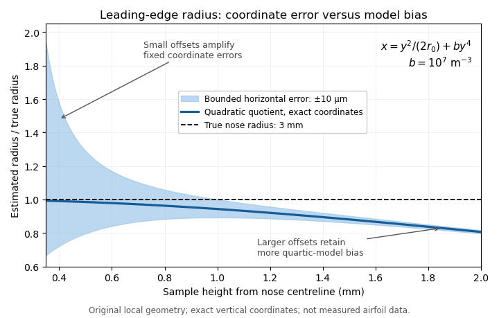
Leading-edge radius quotient for a stipulated quartic nose with true radius 3 mm: small offsets amplify coordinate error, while larger offsets retain more quadratic-model bias. Original calculation; not measured airfoil data.
Details. A least squares fit can combine several points. If the origin and are known and errors are assigned to , minimizing with positive weights givesprovided the denominator and fitted coefficient are positive. This fit does not remove an omitted quartic term; the leading-edge radius fitting window controls the tradeoff between local-model error and coordinate noise. An uncertain nose origin or appreciable errors in both coordinates require a correspondingly expanded fitting model.
A practical geometry check uses calibrated profile coordinates, tests several fitting windows and reports the variation alongside measurement uncertainty. Analytic profiles provide an implementation check: the four-digit family has the known relation .[ref]
Applied Computational Aerodynamics by W. H. Mason. Appendix A, equation (A-5), four-digit leading-edge radius
That family relation validates a calculation on a known profile; it does not determine the radius of an unrelated measured nose.Common-zero cancellation in a drag interaction contrast follows from the coefficients summing to zero. Order the readings as and put . If
then
because . The cancellation is pointwise and does not require to be independent of the residual errors. It requires the same additive offset to enter all four readings on the same scale.
then
because . The cancellation is pointwise and does not require to be independent of the residual errors. It requires the same additive offset to enter all four readings on the same scale.
For finite covariance, the residual contribution to the contrast's variance is . Four independent residual errors with standard deviation give contrast standard deviation , however large the exactly common zero error is. A shared gain error instead multiplies a nonzero true contrast and generally survives.
Run order can also reject some changing zeros. With equally spaced run times in the displayed configuration order, . An additive linear drift therefore cancels. A quadratic drift does not: , leaving . This drift rejection by contrast orthogonality concerns the actual time assignments; a different order can change it.
Normalization can defeat the common-scale assumption. If every dimensional reading has offset but coefficients divide the last reading by twice the dynamic pressure used for the others, the scaled offset no longer has the form . Keeping raw loads and reference readings allows the factorial contrast for aerodynamic interference and its measurement uncertainty to be reconstructed consistently.
AdamW combines the adaptive update of Adam with decoupled weight decay. It maintains exponentially weighted histories of the supplied data gradient and its componentwise square, while applying parameter shrinkage separately. Ilya Loshchilov and Frank Hutter presented the method in their work on decoupling decay from gradient-based regularization.[ref]
Decoupled Weight Decay Regularization by Ilya Loshchilov and Frank Hutter. Version3, Algorithm2, AdamW
For minimization without optional algorithm variants, initialize . In the convention documented by PyTorch, step usesThe product is a Hadamard product; square roots and division are also coordinatewise. Assume , and the stated learning rate . The decay coefficient is . This explicitly fixes epsilon placement and the decay convention.[ref]
AdamW in the PyTorch documentation. PyTorch2.15, algorithm with amsgrad and maximize disabled
The denominators and perform Adam bias correction for zero-initialized histories. For a constant supplied scalar gradient , the corresponding geometric sums give and . Their corrected values are therefore and . The squared-gradient quantity concerns a raw second moment, rather than a centered variance: a constant gradient of 2 has square 4 even though its variance is zero.
For an original first-step example, choose , , , , , and . ThenandThe constants are chosen for transparent arithmetic. Feeding into the same adaptive formulas instead, with no separate shrinkage, would give approximately . That coupled L2 regularization also changes the stored histories. Resuming AdamW therefore requires the relevant optimizer state and step count as well as the parameter values and settings.
AdaGrad is a family of adaptive gradient methods that derives update geometry from accumulated gradient information. Its diagonal form uses a separate cumulative squared-gradient history for each coordinate. John Duchi, Elad Hazan and Yoram Singer's original paper develops diagonal and full-matrix versions, including constrained and regularized settings.[ref]
Adaptive Subgradient Methods for Online Learning and Stochastic Optimization by John Duchi and others. Section1.1, printed pp2122–2124, Eq1 and Eq5
For an unconstrained diagonal specialization, start with and usewhere is the base learning rate, keeps the denominator positive, and is a gradient or suitable subgradient. The additive stabilizer is outside the square root in this declared variant. The accumulator belongs to the optimizer state and must be retained to reproduce later updates.
For an original history example, supply two-coordinate gradientsAfter 100 observations,Choose and . The effective coordinate learning rates are thenAlthough the recent supplied gradients agree, the early large first-coordinate value still strongly reduces its update scale.
Each is nondecreasing, so with fixed and the corresponding effective learning rate is nonincreasing. For a constant nonzero supplied scalar gradient , the history is and the update magnitude isThis tends to zero as the cumulative history grows. Adam instead uses a decaying squared-gradient history, giving old observations a different influence. The choice between these histories is part of the algorithm, rather than merely a different initial learning rate.
Pinned article: Introduction to the OurBigBook Project
Welcome to the OurBigBook Project! Our goal is to create the perfect publishing platform for STEM subjects, and get university-level students to write the best free STEM tutorials ever.
Everyone is welcome to create an account and play with the site: ourbigbook.com/go/register. We belive that students themselves can write amazing tutorials, but teachers are welcome too. You can write about anything you want, it doesn't have to be STEM or even educational. Silly test content is very welcome and you won't be penalized in any way. Just keep it legal!
Intro to OurBigBook
. Source. We have two killer features:
- topics: topics group articles by different users with the same title, e.g. here is the topic for the "Fundamental Theorem of Calculus" ourbigbook.com/go/topic/fundamental-theorem-of-calculusArticles of different users are sorted by upvote within each article page. This feature is a bit like:
- a Wikipedia where each user can have their own version of each article
- a Q&A website like Stack Overflow, where multiple people can give their views on a given topic, and the best ones are sorted by upvote. Except you don't need to wait for someone to ask first, and any topic goes, no matter how narrow or broad
This feature makes it possible for readers to find better explanations of any topic created by other writers. And it allows writers to create an explanation in a place that readers might actually find it.
Figure 1. Screenshot of the "Derivative" topic page. View it live at: ourbigbook.com/go/topic/derivativeVideo 2. OurBigBook Web topics demo. Source. - local editing: you can store all your personal knowledge base content locally in a plaintext markup format that can be edited locally and published either:This way you can be sure that even if OurBigBook.com were to go down one day (which we have no plans to do as it is quite cheap to host!), your content will still be perfectly readable as a static site.
- to OurBigBook.com to get awesome multi-user features like topics and likes
- as HTML files to a static website, which you can host yourself for free on many external providers like GitHub Pages, and remain in full control

Figure 2. You can publish local OurBigBook lightweight markup files to either OurBigBook.com or as a static website.
Figure 3. Visual Studio Code extension installation.
Figure 5. . You can also edit articles on the Web editor without installing anything locally. Video 3. Edit locally and publish demo. Source. This shows editing OurBigBook Markup and publishing it using the Visual Studio Code extension. 
- Infinitely deep tables of contents:




All our software is open source and hosted at: github.com/ourbigbook/ourbigbook
Further documentation can be found at: docs.ourbigbook.com
Feel free to reach our to us for any help or suggestions: docs.ourbigbook.com/#contact