Topics (384k) Articles (398k) Users (410) Discussions (242) Comments (383) Files (13k) New article

Crystallographic resolution describes the spatial detail represented by a diffraction data set and the resulting electron density map. In X-ray crystallography, its conventional numerical measure is the smallest lattice-plane spacing represented by measured reflections. A smaller stated distance means finer nominal resolution.[ref]
Resolution in the IUCr Online Dictionary of Crystallography. Definition: minimum plane spacing and measured diffraction range
From Bragg's law, first-order diffraction at the largest measured glancing angle giveswhere is the X-ray wavelength. For an illustrative wavelength and , the nominal resolution is . At the same wavelength and a maximum angle of15degrees, it is about : collecting smaller-angle reflections alone omits finer spatial information.[ref]
The2000 structure of a bacterial small ribosomal subunit provides a concrete use of the term: its primary report describes refinement to3Å resolution and interprets RNA–protein architecture. That number characterizes the data/model's spatial detail, not an assertion that every atomic coordinate has exactly3Å uncertainty. Noise, missing reflections, directional coverage and model errors still matter.[ref]
Structure of the 30S ribosomal subunit by B. T. Wimberly and others. Abstract: Thermus thermophilus30S subunit refined to3Å
Heavy-atom labeling introduces atoms of relatively high atomic number at ordered crystal sites, giving a strong X-ray scattering contribution so that their signal can supply information for solving its phase problem. In X-ray crystallography, measured intensities constrain the magnitudes of structure factors, while their phases are also needed to reconstruct electron density. A heavy-atom derivative provides an additional measurement linked to a model of the label sites.
Under an ideal single isomorphous replacement model, the derivative keeps the parent structure unchanged apart from the added label contribution. For one reflection, write the complex amplitudes asThe heavy-atom model supplies , while measurements supply and . These are vector constraints in the complex plane; subtracting intensity magnitudes does not directly reveal the protein phase.[ref]
Phasing diagrams in CCP4 Basic Maths for Protein Crystallographers. SIR, two-circle phase construction
For an original example, take , and in consistently scaled amplitude units. If , thenso and . The one-derivative measurement leaves two possible phases. In particular, is not the heavy-atom amplitude3: amplitudes must be combined with their phases.
Multiple isomorphous replacement adds measurements from further derivatives with consistently referenced label positions. These can distinguish the candidate phases in favorable circumstances.[ref]
Phasing diagrams in CCP4 Basic Maths for Protein Crystallographers. MIR, third circle and consistent origin/hand
Large changes in the crystal or protein would violate the stated parent-plus-label model, so derivatization must be assessed rather than assumed to be structurally harmless. Ordered occupancy and useful diffraction matter alongside the chemical act of adding a heavy atom.Crystal isomorphism is a relation between crystal structures that preserves the relevant lattice and structural arrangement while permitting specified atomic replacement or addition. The IUCr definition requires the same space group and unit cell dimensions, with corresponding atom positions and types apart from those substitutions or additions.[ref] Similar external crystal shapes or equal chemical formulas alone do not establish those conditions.
The relation matters experimentally in single isomorphous replacement and multiple isomorphous replacement. A heavy-atom derivative is useful when the unlabeled parent contribution is sufficiently unchanged to write, in a common coordinate convention,Here is the native structure factor and is the reference contribution from the added heavy atoms. If derivatization also changes the parent structure, a more honest decomposition isThe additional term cannot generally be inferred from the heavy-atom label alone. For original complex amplitudes and , the ideal derivative has squared magnitude58. If a structural change contributes , the squared magnitude becomes73. Interpreting that increase solely as extra label scattering would misattribute the change.
Matching unit-cell dimensions is only one test. An original periodic two-site model illustrates why the atomic basis of a crystal matters too. Put identical point scatterers at fractional coordinates and . For the reflection their amplitudes cancel. Moving the second site to without changing the cell dimensions giveswhere is the common atomic scattering factor. At , the magnitude is about rather than zero. The stipulated model is not an experimental derivative; it shows how unchanged lattice spacing can coexist with changed diffraction intensities from shifted atoms.
In actual phasing, crystal isomorphism is an approximation to assess across the measured X-ray diffraction data. The ideal vector-circle constructions assume comparable native and derivative amplitudes and consistently referenced heavy-atom positions.[ref]
Phasing diagrams in CCP4 Basic Maths for Protein Crystallographers. SIR and MIR constructions
Preserved cell metrics support that comparison, but cannot by themselves prove the unchanged-parent assumption.Crystallographic site occupancy is the fraction of a specified atom type present at a modeled site in a crystal structure. Occupancy1 represents full occupation by that type; a fractional value describes an average over the crystal. The IUCr core dictionary distinguishes this fraction from simply listing the site coordinates and constrains the summed occupancies of atom types sharing a physical site.[ref]
A fractional occupancy does not mean that an individual atom has been divided. For an original population example, suppose a site is occupied by the specified atom in750 of1000 equivalent unit cells. Its average occupancy is . More generally, let the crystallographic site multiplicity be equivalent positions per unit cell, each with occupancy0.75. The expected number of those atoms per unit cell iswhere is1 when position is occupied and0 otherwise. Linearity of expectation does not require the occupations to be independent. Correlations and local ordering can differ while the average count remains the same.
If two alternative atom types completely and mutually exclusively fill one site, occupancies0.40and0.60 sum to1. That describes a different model from occupancy0.40 of one type with the rest vacant. Structural alternatives of this kind are associated with crystallographic disorder; occupancy must be interpreted together with the model of what shares the site.
In an ideal structure factor calculation, the contribution of a site is multiplied by its occupancy. For fixed position and atomic displacement parameter, write , where is its full-occupancy complex contribution. A heavy-atom derivative then has . With original values and , occupancy0.5 gives squared amplitude , whereas occupancy1 gives . The native value is25. Intensity changes are therefore not simply proportional to occupancy, because the added amplitude interferes with the parent amplitude.
The IUCr dictionary for multiple isomorphous replacement records occupancy separately for a heavy-atom site in each derivative.[ref]
Heavy-atom site occupancy in the PDBx/mmCIF Dictionary.
A refined fraction concerns that structural site and scattering model; it is not by itself a general measurement of bulk chemical purity._phasing_MIR_der_site.occupancyCrystallographic site multiplicity is the number of distinct equivalent positions generated from one representative site by the space group within the conventional unit cell. It is a property of the Wyckoff position. If the site-symmetry group leaves a representative position fixed, fewer distinct positions are generated than at a general site.[ref]
Atom-site symmetry and disorder in the IUCr core CIF dictionary.
_atom_site_site_symmetry_multiplicity, DefinitionThe relation can be writtenwhere is the general-position multiplicity and is the order of the site-symmetry group. For an original compatible example, general multiplicity8 and site-symmetry order2 give .
Multiplicity is distinct from crystallographic site occupancy . For one atom type represented at equivalent positions, its average contribution to the atom count per unit cell isA multiplicity8 site occupied to0.25 contributes2 atoms per cell on average. A fully occupied multiplicity4 site contributes4. If these are separate inequivalent sites for the same element, their total contribution is6.
Full occupancy at a symmetry-special site is still , rather than automatically a fractional value. The symmetry reduction is already counted by . Dividing occupancy again by the site-symmetry order would count that reduction twice. These distinctions connect a list of representative coordinates to the chemical contents of the unit cell.
Crystallographic disorder is variation in atomic positions, orientations or chemical occupation that is represented by an average crystal structure rather than one perfectly repeated local arrangement. A split-site disorder model can describe alternative positions with fractional crystallographic site occupancies. The IUCr disorder-group convention distinguishes atoms present together in one configuration from mutually alternative configurations.[ref]
Atom-site symmetry and disorder in the IUCr core CIF dictionary.
_atom_site_disorder_group, jointly occupied sites and alternative groupsFor an original single-atom model, suppose an atom occupies position0 along an axis with probability0.6 and position with probability0.4. ThenAt , the mean is and the variance is . There need be no atom at the mean position in any individual configuration. Fitting only an average position with a large atomic displacement parameter can conceal this distinction.
The same average occupation could arise from different unit cells adopting different configurations, from motion among configurations during measurement, or from a mixture of these effects. A static average alone does not determine an interchange rate.
Experimental interpretation therefore combines the electron density map, the allowed chemical geometry, occupation constraints and other evidence. Weak or broadened density should not automatically be assigned one specific dynamic mechanism.
An atomic displacement parameter describes the spread of an atom's modeled position about its mean in a crystal structure. An isotropic atomic displacement parameter represents equal spread in all directions; an anisotropic atomic displacement parameter uses a directional matrix. These parameters can reflect thermal motion, unresolved static variation and limitations of the refinement model, rather than temperature alone.
For isotropic Cartesian displacement, let be the mean-square displacement of one component, in squared angstroms. The conventional alternative parameter isThe IUCr dictionary gives both conventions and prefers reporting .[ref]
Atomic displacement parameters in the IUCr core CIF dictionary. Definitions of U/B isotropic or equivalent displacement parameters and their conversion
For an original numerical example, givesThe second value is the root-mean-square spread along one Cartesian direction. Under isotropy the three-dimensional mean-square displacement is , so the corresponding radial root-mean-square spread is about .
This spread is not the same as uncertainty in the refined mean coordinate. Nor does doubling by itself prove that an atom's temperature doubled. Crystallographic disorder, imperfect data and a different structural model can affect the fitted parameter. Interpretation requires the experimental and modeling context.
An electron density map is a spatial reconstruction of electron density, typically displayed as a grid or contours. In X-ray crystallography, a beam scattered by a crystal produces a diffraction pattern: measured intensities constrain structure factor magnitudes, while crystallographic phases are also required for reconstruction. Coordinates and experimental data are combined in common model-assessment maps.[ref]
Electron Density Maps and Coefficient Files at RCSB PDB. Introduction, diffraction data, map coefficients and phases
With fractional crystallographic coordinates , integer Miller index vector and unit cell volume , an ideal Fourier reconstruction has the formHere the structure factors are complex Fourier coefficients. Finite data and uncertain phases limit the reconstructed detail; this is part of the phase problem, not simply an issue of drawing contours more finely.
An original one-dimensional example makes the phase information visible:Both profiles have the same Fourier coefficient magnitudes, but their maxima occur half a period apart. Squared magnitudes alone cannot distinguish them.
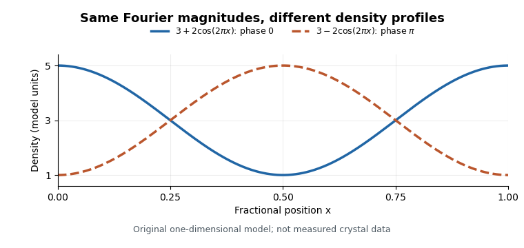
Equal Fourier magnitudes can give different density profiles
. Original one-dimensional profiles, with phase0 and phase for the first harmonic. Both have mean3 and first-harmonic coefficient magnitude1. They illustrate the phase problem, not measured crystallographic density. Details.An electron density map is also distinct from a macromolecular structural model fitted to it. A difference electron density map can highlight disagreement between observed and model-predicted scattering. Common map coefficients already incorporate information from the model, so the resulting map is not wholly independent confirmation of every modeling choice.[ref]
Electron Density Maps and Coefficient Files at RCSB PDB. Introduction, observed/calculated maps and difference maps
For a wrench with nonzero resultant force and moment about a stated point , its wrench pitch isIt has units of length: torque divided by force. It measures the signed moment remaining parallel to the resultant, per unit force. The force/moment representation and its frame transformations are developed in the primary robotics text’s wrench supplement.[ref]
Modern Robotics: Mechanics, Planning, and Control by Kevin M. Lynch and Frank C. Park. §3.4, Wrenches, transcript: force/moment six-vector, reference-frame change and power pairing
The wrench pitch does not depend on the moment origin. Moving from to , with displacement expressed in the same axes, gives . Taking the dot product with removes the added term because . A common rotation of both vectors also preserves the ratio. Scaling every applied load by the same nonzero scalar leaves unchanged.
The central axis of a wrench makes the meaning visible. DefineThe vector triple-product identity givesEvery point on the line has that same parallel residual moment. This line also minimizes the moment magnitude over all choices of origin: the perpendicular part can be removed, while the invariant parallel part cannot. The minimum is .
For an original example, let and . Then and . Translating the moment origin to that point leaves : a axial force together with a axial force couple. No relocation of a single force can eliminate this remaining couple.
If with , the central-axis moment vanishes and one force on that line reproduces the external load system. If and the moment is nonzero, the load is a pure force couple; the formula for is undefined. An infinite-pitch description is a limiting screw-theory convention, not a finite value supplied by this quotient. Both zero force and zero moment give the zero wrench and no distinguished axis.
A proposed load-sensor check combines a known force on an offset line with a known parallel couple. Recompute moments about several origins and compare the resulting values. Errors in origin translation can corrupt the moment components while the exact invariant remains fixed; near zero resultant force, the division by makes pitch sensitive to measurement error. This geometric load parameter is not automatically a physical screw’s thread spacing.
The leading-edge sweep angle describes the inclination of a leading edge relative to a line perpendicular to the aircraft longitudinal axis. On one half-wing, take positive aft and positive outward. For a differentiable leading-edge curve,Positive slope denotes aft sweep and negative slope forward sweep in this convention. A coordinate reference must be supplied before the sign has meaning.[ref]
Applied Computational Aerodynamics by W. H. Mason. Appendix A, planform coordinate sketch and equation (A-97)
For a straight edge on a symmetric wing, let its tip be displaced aft from the root by and let be the full wingspan. ThenFor an original example, and give . Incorrectly using the full span as the root-to-tip run would give . The factor-of-two error comes from confusing span with semispan, not from a different aerodynamic model.
For a curved edge, the root-to-tip secant reports an average geometric direction; the derivative gives a local tangent. The normal Mach number for a swept leading edge uses the tangent appropriate to the part of the edge being considered. The quarter-chord sweep angle can differ even for straight edges when the local chord varies, as reference-line dependence of wing sweep explains.
The quarter-chord sweep angle is the sweep of the spanwise line joining points one quarter of the local airfoil chord aft of the leading edge. It is a wing-planform reference direction, not the angle of attack and not the mean aerodynamic chord's quarter-point location.
For chordwise coordinate increasing aft,The reference-line dependence of wing sweep gives the general relation. On a straight-edged trapezoidal wing with full wingspan , root chord and tip chord ,Mason explicitly relates sweep at different chord fractions in the planform geometry.[ref]
For an original inverse calculation, let , , and . The leading-edge tangent is , giving . With the root leading edge at , the root quarter-point is at . The tip quarter-point is aft of that origin, while the tip leading edge is farther forward.
This calculation uses the full span in the chord-gradient formula and the semispan in the root-to-tip displacement. It also shows why the normal Mach number for a swept leading edge needs its own leading-edge direction: a reported fifteen-degree quarter-chord sweep does not make the leading edge fifteen degrees.
Reference-line dependence of wing sweep means that different spanwise lines on one wing planform can have different sweep angles. Naming the line is therefore necessary to specify the geometry. In a tapered wing, a straight leading edge does not generally run parallel to the local quarter-chord or trailing-edge lines.
Let increase aft and run outward on one half-wing. If the local airfoil chord is , the line at a fixed chord fraction isFor two fixed fractions , subtraction givesThis is a relation between tangents of angles, not the angle difference itself. Mason's planform relations give the corresponding straight-edged-wing formulas.[ref]
For an original example, take wingspan , root chord and tip chord , varying linearly. Then . Choose a leading-edge slope . Its leading-edge sweep angle is , but its quarter-chord sweep angle obeys . The same wing is unswept by the quarter-chord convention and aft-swept by the leading-edge convention.
For constant chord, and the local angles agree at all chord fractions. For curved edges or nonlinear taper, the angles can also vary with , making a local tangent distinct from a root-to-tip secant. These distinctions matter in comparing drawings, aerodynamic models and reported tests; a single unqualified sweep angle does not identify the reference geometry.
The normal Mach number for a swept leading edge is the incoming velocity component perpendicular to that edge divided by the local speed of sound. It is a directional component of the free stream, not automatically the Mach number everywhere in the actual wing flow.
Let be a unit tangent along a straight leading edge, let be the incoming velocity, and let be the speed of sound. Vector projection givesFor a planar wing with flow aligned with its longitudinal reference direction and leading-edge sweep angle , the component along the edge is . ThusThe cosine is nonnegative in the usual sweep range between and degrees. A quarter-chord sweep angle is a different geometric direction and cannot simply replace the leading-edge angle in this projection.
For an original example, and give . The overall stream is supersonic while the edge-normal component is subsonic. For , the boundary occurs at , about for . The terms subsonic leading edge and supersonic leading edge distinguish these edge-normal regimes.
Using the component as a predictor of an entire finite-wing flow adds assumptions. Thickness, finite span, angle of attack and interference with the fuselage can all matter. Whitcomb's pressure and wake measurements found that shock-associated changes with sweep did not follow the simple cosine shift exactly.[ref]
An Investigation of the Effects of Sweep on the Characteristics of a High-Aspect-Ratio Wing in the Langley 8-Foot High-Speed Tunnel by Richard T. Whitcomb. NTRS author abstract, comparison of observed changes with the cosine factor
The projection itself is exact for the stated vectors; the reduction of a three-dimensional aerodynamic problem to that single component is the approximation.An image mask is a function on image coordinates specifying which pixels or regions are retained or weighted. A binary mask selects a region, while a soft mask takes intermediate weights. Applying the mask pointwise gives for image intensity .
For example, a mask equal to one inside a disk and zero outside retains only that disk of an image. An edge with fractional weights can smooth the transition. The mask describes location or weighting, rather than assigning a new color to every retained pixel.
In Fourier analysis, multiplication by a window function in the image plane corresponds to convolution in frequency, with the constant depending on the Fourier convention. A sharp binary boundary can therefore introduce broad high-frequency contributions. This explains why cropping and spectral filtering have different mathematical effects.
The coherent gain of a discrete window function is its mean coefficient:It describes the amplitude scaling of a coherent complex tone under the chosen DFT normalization. Window coefficients and their normalization must be specified; a window's name alone does not fix every finite-length convention.[ref]
LabVIEW Analysis Concepts by National Instruments. Printed pages 5-20–5-24, periodic/symmetric windows and coherent-gain scaling
For , multiply by and evaluate the unnormalized discrete Fourier transform at the exact tone bin:Thus recovers when . This result is exact for this complex-tone model. A real cosine also has a negative-frequency component; the usual doubled one-sided amplitude requires that its contribution to the chosen positive-frequency bin be absent or separately accounted for.
A rectangular window has . The periodic Hann window has for . Its coherent bin therefore has half the unwindowed amplitude before correction. The symmetric endpoint convention , for , instead gives . At this is , so blindly multiplying by two is not the exact correction for that convention.
Coherent gain does not correct every amplitude error. An off-bin tone samples the window's frequency response away from its maximum, and a DC-removing window with zero sum has no usable gain correction at all. Coherent sampling, leakage and window normalization are distinct conditions.
Noise uses a different scaling. For independent equal-variance samples, a weighted DFT bin's noise variance is proportional to , not . This motivates equivalent noise bandwidth in bins,which is for a periodic Hann window with . The manufacturer's table lists both coherent gain and noise bandwidth rather than treating one as a substitute for the other.[ref]
A Hann window tapers a record with a raised cosine. For the endpoint-symmetric convention with ,It vanishes at the two stored endpoints. A periodic convention instead uses denominator , corresponding to sampling one cosine period without storing its repeated endpoint. SciPy's primary documentation distinguishes these with
sym=True and sym=False; the default is symmetric.[ref] The adjacent Hanning window alias also supports the terminology used in older instrument documentation.An original short-array example makes the difference concrete. At , the symmetric coefficients are , while the periodic coefficients are . Their means are and . A symmetric even-length array need not contain a coefficient equal to one, despite the nominal raised-cosine peak.
The coherent gain of a window is . It equals for the periodic Hann convention with , and for the symmetric convention with . A coherent complex tone gives windowed DFT magnitude at its exact bin, so amplitude recovery must use the chosen coefficient sum.
For the periodic convention, its discrete-time Fourier transform is obtained from the rectangular window transform by modulation:The first central zeros lie at for the usual case, twice as far from the center as the rectangular window's first zeros. Smooth tapering reduces distant sidelobes while widening the central feature. Nearby frequencies and a weak component far from a strong one can therefore favor different window choices.
Noise normalization is another distinction. For , the periodic Hann coefficients obey and , giving equivalent noise bandwidthin DFT bins. The manufacturer's table lists both coherent gain and noise bandwidth.[ref] Correcting a coherent amplitude does not make noise behave as though the rectangular weights had been used.
The original comparison below evaluates the finite 64-sample periodic Hann and rectangular coefficients at a dense frequency grid, normalizing each response by its own coefficient sum. The extra frequency samples display the same finite-record transform more finely; they do not create a longer observation.
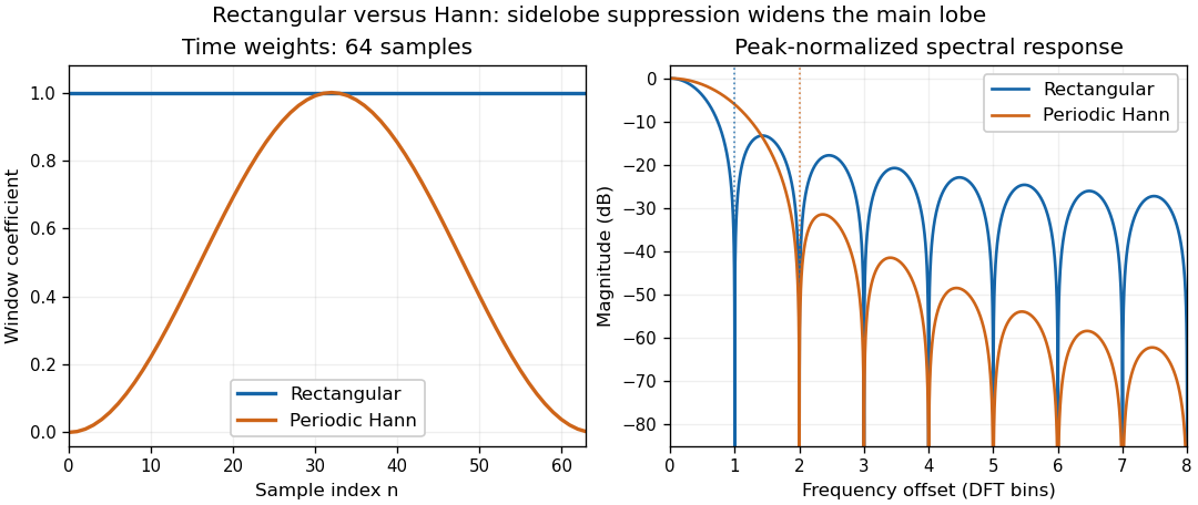
Original 64-sample rectangular and periodic Hann windows: lower distant sidelobes accompany a wider central lobe
. Each spectral curve is normalized to its own coherent peak. The horizontal frequency axis is measured in DFT-bin offsets. The first positive zeros are at one bin for the rectangular window and two bins for the periodic Hann window. Details.A rectangular window keeps all samples in a selected finite record with equal weight and sets the signal outside it to zero. For discrete samples, for and zero otherwise. Calling this no taper does not remove the effect of having a finite record. SciPy's primary implementation documentation identifies the boxcar and rectangular window as this same all-ones choice.[ref]
Its discrete-time Fourier transform at frequency in cycles per sample is a finite geometric sum:At integer , the limiting value is . The first zeros surrounding the central maximum are at , so the central zero-to-zero width is . The phase factor depends on the record's time origin; the magnitude response does not.
For a continuous centered record of duration , on has transformwhere the normalized sinc function is . Multiplication by the finite window spreads a sharp spectral component according to this response, producing spectral leakage.
An original finite-record example quantifies an off-bin amplitude error. A complex tone of amplitude lying half a DFT bin from the nearest sampled frequency has normalized responseAt the ratio is about , or relative to the coherent peak. The coherent gain of a window is still one; it does not correct this scalloping loss. Zero-padding samples the same frequency response more densely rather than lengthening the measured record.
For independent equal-variance sample noise, rectangular weighting has equivalent noise bandwidth of one DFT bin under the usual coherent-amplitude normalization. A Hann window suppresses distant sidelobes but changes the central width and noise scaling. The primary analysis manual reports these separate window properties rather than one universal best window.[ref]
A proposed test records a known sinusoidal input with an integer and then a non-integer number of cycles in the same record length, holding the sampling rate and amplitude fixed. Compare the raw DFT bins and the continuous window response. This separates finite-record leakage and bin placement from aliasing, which involves a different sampling ambiguity.
The equivalent noise bandwidth of a finite window is the width of an ideal rectangular frequency response that passes the same white-noise power when both responses have the same peak gain. It quantifies noise collected by a spectral amplitude estimate, rather than the separation needed to distinguish two tones. For real coefficients with nonzero sum and sampling frequency , is in hertz; is in bins of an -sample record. The primary software documentation gives as the exact conversion factor between its squared spectrum and power-spectral-density scalings.[ref]
An original variance derivation explains the formula. Let independent zero-mean sample noise have variance , and form the complex amplitude estimate at frequency ,Cross terms vanish by the independence and zero means, soThe flat two-sided input noise spectral density is . Integrating it over the peak-normalized window response gives the same result by Parseval identity. A one-sided real-signal convention folds negative-frequency power into positive frequencies; factors of two must be handled consistently, rather than changing the window’s bandwidth ratio.
For a rectangular window, and , giving . For the periodic Hann window with , the cosine sums give and , hence . These agree with the instrument manual’s tabulated values.[ref]
For an original numerical comparison, take and , so the original frequency grid spacing is . Rectangular and periodic Hann bandwidths are respectively and . With independent sample noise of standard deviation , the RMS magnitude of the zero-mean complex noise estimate is for rectangular weighting and about for Hann weighting. The latter variance is 1.5 times greater, despite Hann’s lower distant sidelobes. It is the RMS complex-error magnitude, not automatically the standard deviation of a positive spectral-magnitude display.
Zero padding leaves , the actual window coefficients and unchanged. If a 256-sample Hann record is padded to 1024 points, the display spacing becomes and the same bandwidth spans six displayed bins. Replacing by the padded FFT length in a formula while leaving the coefficient sum unchanged confuses these two bin units.
The noise covariance between windowed Fourier bins also matters when combining several spectral values: a taper can correlate neighboring estimates. Bandwidth alone does not specify their joint statistics, and colored noise requires weighting its actual spectral density. A proposed check repeats the same estimator on independent synthetic noise records with known variance, then on measured noise with a characterized acquisition response, comparing empirical mean squared complex error with the formula. Report window convention, detrending, one-sided/two-sided scaling and record duration so the test can be reproduced.
Scalloping loss is the underestimate of an isolated sinusoidal amplitude caused by measuring it only at the nearest sampled discrete Fourier transform frequency, after correcting the window’s coherent amplitude scale. An off-grid tone is evaluated away from the maximum of the window response. This differs from the coherent gain of a window, which describes the response at the correctly centered frequency. The instrument manual treats amplitude scaling and off-bin errors separately.[ref]
Let be a finite real window with positive sum, and let , where is the nearest unpadded DFT bin and . Write . The coherent-gain-corrected bin magnitude relative to isHere is a positive loss when . The half-bin amplitude response of a window evaluates this ratio at the largest nearest-bin offset. Other tones, noise and the negative-frequency image of a real sinusoid can also affect a measured peak; the derivation isolates one complex tone.
For a rectangular window, its geometric-sum transform givesFor , the half-bin ratio is about and the loss about . An amplitude-one tone exactly centered on a bin is recovered as one, while the same tone shifted by half a bin gives only about at either nearest bin. Dividing by coherent gain cannot remove this offset dependence.
For the periodic Hann window, usewhere is the rectangular response. At , this gives a half-bin ratio about , or loss. The smaller nearest-bin error comes with a wider main lobe and a larger equivalent noise bandwidth; window choice affects several measurement properties at once.
Zero padding reduces the nearest-grid offset without changing the measured record. Padding to points makes the nearest offset at most in original-bin units. With and , the rectangular response at that worst offset is about , a loss of only . This is denser sampling of the same discrete-time Fourier transform, not extra physical frequency resolution. A fitted peak can reduce a grid error too, but its signal model and noise sensitivity must be stated.
A proposed analyzer test holds tone amplitude fixed while sweeping frequency through one bin interval, retaining record length, sampling rate and window. Divide out coherent gain, plot the measured peak versus fractional-bin offset, and compare with the exact response above. Include phase and nearby-tone checks for a real signal. Summing spectral powers instead answers an energy question and requires its own bandwidth normalization; it should not silently replace this single-bin amplitude definition.
Pinned article: Introduction to the OurBigBook Project
Welcome to the OurBigBook Project! Our goal is to create the perfect publishing platform for STEM subjects, and get university-level students to write the best free STEM tutorials ever.
Everyone is welcome to create an account and play with the site: ourbigbook.com/go/register. We belive that students themselves can write amazing tutorials, but teachers are welcome too. You can write about anything you want, it doesn't have to be STEM or even educational. Silly test content is very welcome and you won't be penalized in any way. Just keep it legal!
Intro to OurBigBook
. Source. We have two killer features:
- topics: topics group articles by different users with the same title, e.g. here is the topic for the "Fundamental Theorem of Calculus" ourbigbook.com/go/topic/fundamental-theorem-of-calculusArticles of different users are sorted by upvote within each article page. This feature is a bit like:
- a Wikipedia where each user can have their own version of each article
- a Q&A website like Stack Overflow, where multiple people can give their views on a given topic, and the best ones are sorted by upvote. Except you don't need to wait for someone to ask first, and any topic goes, no matter how narrow or broad
This feature makes it possible for readers to find better explanations of any topic created by other writers. And it allows writers to create an explanation in a place that readers might actually find it.
Figure 1. Screenshot of the "Derivative" topic page. View it live at: ourbigbook.com/go/topic/derivativeVideo 2. OurBigBook Web topics demo. Source. - local editing: you can store all your personal knowledge base content locally in a plaintext markup format that can be edited locally and published either:This way you can be sure that even if OurBigBook.com were to go down one day (which we have no plans to do as it is quite cheap to host!), your content will still be perfectly readable as a static site.
- to OurBigBook.com to get awesome multi-user features like topics and likes
- as HTML files to a static website, which you can host yourself for free on many external providers like GitHub Pages, and remain in full control

Figure 2. You can publish local OurBigBook lightweight markup files to either OurBigBook.com or as a static website.
Figure 3. Visual Studio Code extension installation.
Figure 5. . You can also edit articles on the Web editor without installing anything locally. Video 3. Edit locally and publish demo. Source. This shows editing OurBigBook Markup and publishing it using the Visual Studio Code extension. 
- Infinitely deep tables of contents:




All our software is open source and hosted at: github.com/ourbigbook/ourbigbook
Further documentation can be found at: docs.ourbigbook.com
Feel free to reach our to us for any help or suggestions: docs.ourbigbook.com/#contact