Auxin response factor 1, historically abbreviated ARF1 in this plant context, is a transcription factor characterized for its ability to bind auxin response elements. The 1997 report isolated it using a yeast one-hybrid assay and related its DNA-binding specificity to sequences that conferred an auxin-responsive transcriptional effect.^[ref]

The study identified an amino-terminal DNA-binding domain and a distinct carboxyl-terminal region associated with interactions between proteins. This supplies a concrete example of modular regulation: contacting a target DNA sequence and contacting another regulator can involve different parts of one protein.^[ref]

Experiments with DR5 auxin response elements also showed ARF1 binding and interactions with Aux/IAA proteins. Those observations connect a named factor to a defined regulatory system. They do not turn every auxin response factor into the same protein, nor make DNA binding alone a complete account of the resulting gene expression.^[ref]

The DR5 auxin response element is a synthetic regulatory DNA arrangement containing repeated auxin response elements. When used to control a reporter gene, it contributes the responsive regulatory part of a DR5 auxin response reporter. The DNA element and the measurable reporter product are different parts of that system.^[ref]

The original study compared DR5 with natural regulatory sequences and found strong auxin-responsive expression in the tested plant systems. It also connected binding by auxin response factor 1 with regulatory effects involving Aux/IAA proteins. This made DR5 useful for studying responsive transcription, rather than establishing a direct physical measurement of auxin concentration.^[ref]

An illuminating experimental distinction is between asking whether a protein recognizes this DNA arrangement and asking whether a reporter is expressed in a particular cell. The first concerns molecular binding; the second also depends on the surrounding regulatory system and reporter behavior. A repeated regulatory element can therefore be a sensitive response tool without being a universal hormone-concentration scale.

An isotropic atomic displacement parameter describes the same mean-square positional displacement along every Cartesian direction in a crystal structure. Its Cartesian displacement covariance matrix isThus $U_{\mathrm{iso}}$ is a one-component variance, in squared angstroms, rather than a displacement length. The alternate conventional parameter is $B=8{\pi }^2{U}_{\mathrm{iso}}$.^[ref]

For an original example, $U_{\mathrm{iso}}=0.020{\mathring{\mathrm{A}}}^2$ givesThe radial root-mean-square displacement is instead $\sqrt{3U_{\mathrm{iso}}}\simeq 0.245\mathring{\mathrm{A}}$ because it includes three components.

For a centered isotropic normal distribution, the structure factor amplitude attenuation at reciprocal-vector magnitude $s$, measured in cycles per angstrom, isAt $s=1{\mathring{\mathrm{A}}}^{-1}$, the stated example gives $T\simeq 0.674$ and squared-amplitude attenuation $T^2\simeq 0.454$. Amplitude and intensity attenuation are therefore distinct, even in this simple Gaussian model.

An equivalent isotropic atomic displacement parameter can also summarize an anisotropic atomic displacement parameter by its Cartesian trace divided by3. Such an average can appear in the same CIF field as a genuinely isotropic parameter, but does not assert equal directional spread.^[ref]

An anisotropic atomic displacement parameter describes direction-dependent positional spread about an atom's mean position in a crystal structure. In Cartesian coordinates a physical displacement model has a symmetric covariance matrixThe six independent entries have units of squared length. The crystallographic components stored in CIF use a cell-dependent convention, including reciprocal-cell lengths in the structure factor attenuation; they must be transformed before being interpreted as Cartesian covariance entries.^[ref]

For an original Cartesian example, letThe principal root-mean-square displacements are0.1,0.2 and0.3 angstroms. An atomic displacement ellipsoid displays those preferred directions; its displayed boundary also depends on the chosen probability level. Rotating the coordinate axes generally introduces off-diagonal entries without changing the physical spread or eigenvalues.

Under a centered multivariate normal distribution for $\mathbf{u}$, its contribution to the scattering amplitude is multiplied bywhere $\mathbf{s}$ is the Cartesian reciprocal vector in cycles per unit length. Thus reflections probing different directions can distinguish directional spread. A physically valid covariance is a positive semidefinite matrix.

The equivalent isotropic atomic displacement parameter is $U_{\mathrm{eq}}=\mathrm{tr}(U)/3$ in Cartesian coordinates. In this example it is $0.04667{\mathring{\mathrm{A}}}^2$; that average does not make the original distribution isotropic. Positional spread can include unresolved static variation as well as motion, and differs from uncertainty in the refined mean coordinate.^[ref]

The equivalent isotropic atomic displacement parameter summarizes an anisotropic atomic displacement parameter by the average mean-square displacement along three perpendicular Cartesian directions:It has units of squared length. The corresponding equivalent $B$ parameter is $B_{\mathrm{eq}}=8{\pi }^2{U}_{\mathrm{eq}}$. The CIF field for isotropic displacement may contain either a genuinely isotropic atomic displacement parameter or this anisotropic summary.^[ref]

For an original example, take a Cartesian displacement covariance matrixThen $U_{\mathrm{eq}}=0.020{\mathring{\mathrm{A}}}^2$ and $B_{\mathrm{eq}}\simeq 1.579{\mathring{\mathrm{A}}}^2$. The principal root-mean-square displacements are0.1,0.1 and0.2 angstroms. A genuinely isotropic matrix $0.020I$ has the same equivalent parameter but a different directional distribution.

The trace is invariant under Cartesian rotations, so the average does not depend on the laboratory orientation. In an oblique crystallographic basis, however, the raw diagonal entries of the stored displacement matrix do not in general have this Cartesian interpretation. The cell geometry must enter the conversion before taking the physical trace.^[ref]

This scalar is convenient for comparisons and tabulation, but discards directional information displayed by an atomic displacement ellipsoid. Equality of equivalent parameters therefore neither establishes isotropy nor proves that two sites have the same displacement distribution.

Aspartate denotes an anionic form of aspartic acid. A common biochemical example is the L-configured monoanion, with two carboxylate groups and one positively charged amino group. Its formula is ${\mathrm{C}}_4{\mathrm{H}}_6\mathrm{N}{\mathrm{O}}_4^{-}$ and its net charge is $-1$.^[ref]

The charge count isHaving both positive and negative groups therefore does not imply a zero total charge. Compared with neutral aspartic acid, formation of this conjugate base removes a proton; it does not change the four-carbon connectivity or, by itself, reverse the L/D stereochemistry.

An illustrative acid–base comparison keeps these questions separate. For one protonation step in a dilute solution, the Henderson-Hasselbalch equation gives $[\mathrm{base}]/[\mathrm{acid}]\simeq 10^{\mathrm{pH}-\mathrm{p}{K}_a}$. One pH unit above that step's $\mathrm{p}{K}_a$ gives a ratio of about ten. This is a symbolic illustration, not a numerical assignment of the molecule's several dissociation constants. Specifying ionic form, pH and stereochemistry is more informative than treating every use of the name aspartate as one context-free structure.

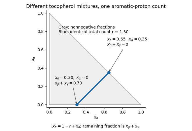
Mixture ambiguity in aromatic-proton counts is the inability of a total aromatic proton nuclear magnetic resonance integral to identify all components of a tocopherol mixture. The named substitution patterns leave zero, one, one and two aromatic hydrogens in alpha-tocopherol, beta-tocopherol, gamma-tocopherol and delta-tocopherol, respectively.^[ref]

Let their mole fractions be $x_{\alpha },x_{\beta },x_{\gamma },x_{\delta }$. Under an ideal quantitative response model, an aromatic integral normalized per tocopherol molecule givesThe normalization requires an independently established molecular amount or an equivalent valid calibration. A raw integral alone is not automatically a hydrogen count per molecule. This model also assumes that the selected response includes the relevant aromatic protons with compatible quantitative acquisition conditions.

There are four unknown fractions but only two displayed linear constraints. In particular, exchanging any allowed amount of beta-tocopherol for gamma-tocopherol preserves both constraints: their equal counts cannot distinguish these constitutional isomers.

An original feasible-range calculation makes the remaining ambiguity explicit. Setting $d=x_{\delta }$ givesNonnegative fractions implyFor $r=1.30$, any $d$ between $0.30$ and $0.65$ can fit. The first endpoint has no alpha-tocopherol and a combined beta/gamma fraction of $0.70$; the second has alpha fraction $0.35$ and no beta/gamma component. Intermediate values and beta/gamma exchanges produce further mixtures with the same count.

Resolving additional chemical shifts or using an independently calibrated chromatography measurement can provide new component-sensitive evidence. Repeating the same total integral more precisely only narrows the uncertainty around $r$; it does not add the missing independent composition constraints. The calculation expresses structural possibilities from the named molecules, not an assignment of measured peak positions.

The area density of a smooth surface with Riemannian metric $g$ is the positive coordinate-invariant rule for measuring surface area. In a chart $(u,v)$, with first fundamental form $Ed{u}^2+2Fdudv+Gd{v}^2$, it isUnder a coordinate change with Jacobian matrix $J$, the metric matrix becomes $J^{T}gJ$, so its determinant acquires $(\det J{)}^2$. The square root therefore transforms by $|\det J|$, exactly the density transformation needed for an unsigned integral.

For a parametrized surface $X(u,v)\subseteq {\mathbb{R}}^3$, the same coefficient is $|X_u\times X_v|$. A radius-$R$ sphere in polar coordinates has density $R^2\sin \theta |d\theta d\phi |$, giving total area $4\pi R^2$. Unlike an oriented area two-form, an area density exists on a Möbius band; reversing orientation does not negate area.

Aperture-scan separation of direct and diffuse nail transmission estimates the directly collected and diffusely transmitted fractions of light by changing detector acceptance while keeping the nail plate and illumination fixed. Separation depends on a stated angular model: a change in aperture is an experimental control, not a direct label attached to every photon.

In the original constant-diffuse-radiance model, let $Y_j=T_d+{\eta }_j{T}_s+{ϵ}_j$, where $T_d$ is the fully accepted direct fraction, $T_s$ the total diffuse fraction and ${\eta }_j$ the known diffuse acceptance. For a coaxial circular opening, the geometric approximation gives ${\eta }_j=a_j^2/(a_j^2+r^2)$. Two distinct acceptances giveThe distinction between these components is identifiable within this model only when the acceptances differ.

Suppose ${\eta }_1=0.20$, ${\eta }_2=0.50$, $Y_1=0.056$ and $Y_2=0.080$. The fitted fractions are ${\hat{T}}_s=0.08$ and ${\hat{T}}_d=0.04$. If independent signal errors each have standard uncertainty $\sigma =0.002$, with acceptance uncertainty temporarily neglected, linear propagation givesandThe resulting uncertainties are about 0.00943 and 0.00359. Their negative covariance matters when adding the components: the total-transmission uncertainty is about 0.00629, rather than the value obtained by incorrectly treating the fitted components as independent.^[ref]

Additional apertures give a straight-line fit of $Y$ against $\eta$, with intercept $T_d$ and slope $T_s$. Weighted least squares can use independently characterized signal uncertainties. Systematic curvature would challenge the assumed angular law or fixed direct-beam acceptance. A plausible line alone does not prove that a finite source, changing geometry or residual fluorescence has been modeled correctly.

The primary nail-transmission study collected transmitted light using an integrating sphere, monochromator and photodiode.^[ref] The aperture scan here is an original proposed comparison, not a procedure or angular scattering law reported in that experiment.

The virtual basal ring is the geometric reference formed from the lowest attachment points of the three aortic valve leaflets. It specifies a basal plane of the aortic root; it is not the entire crown-shaped tissue attachment represented by the anatomical aortic annulus.^[ref]

Three noncollinear landmarks determine a plane. For landmark position vectors ${\mathbf{p}}_1,{\mathbf{p}}_2,{\mathbf{p}}_3$, a normal isThe reference plane then obeys $\mathbf{n}\cdot (\mathbf{x}-{\mathbf{p}}_1)=0$. Near-collinear landmarks make $\Vert \mathbf{n}\Vert$ small, illustrating geometrically why landmark identification affects orientation. These equations construct a reference, not a ring of newly discovered tissue.

A plane alone also supplies no unique anatomical outline. Three points can define a circumcircle, but choosing that circle is a modeling convention; the actual lumen outline in that plane can be noncircular. For an original ellipse with semiaxes 15 and 10 mm, the enclosed area is $150\pi$ mm${}^2$ and the equal-area circular diameter is $2\sqrt{150}\simeq 24.49$ mm. Neither the 30 mm major diameter nor the 20 mm minor diameter equals that number.

The virtual basal ring is useful because it gives different images a specified basal reference. A measurement must still identify its landmarks, outline, cardiac cycle phase and diameter or area convention. It should not silently substitute the sinotubular junction or the longer three-dimensional leaflet attachment path for this basal reference.

The aortic root is the proximal aorta associated with the aortic valve, extending from the basal leaflet reference toward the sinotubular junction. It includes the leaflet-bearing region and the bulges called aortic sinuses, and gives origin to the coronary arteries. It connects the left ventricular outflow tract to the tubular ascending aorta.^[ref]

The boundaries answer different anatomical questions. The virtual basal ring is constructed from basal leaflet attachment landmarks, whereas the sinotubular junction marks the distal transition. The three-dimensional leaflet attachments are crown-shaped, so the word aortic annulus requires a stated convention. The anatomical account by Robert H. Anderson emphasizes this terminology problem.^[ref]

An original volume balance shows why the aortic root is more than a named length of Pipe. Let $Q_{\mathrm{in}}$ enter through the aortic valve, $Q_{\mathrm{out}}$ leave toward the ascending aorta, and $Q_{\mathrm{cor}}$ denote total outflow into the coronary arteries. For blood treated as incompressible,Stipulated mean rates over 0.1 s of 100, 80 and 5 mL/s give a 1.5 mL increase in stored volume. Over a repeating cardiac cycle, zero net accumulation instead requires equal integrated inflow and total outflow. Instantaneous equality is unnecessary if the region changes volume.

Measurement likewise requires a named level. The primary anatomical exposition illustrates separate basal, sinus and sinotubular junction diameters in an echocardiography view.^[ref] Reporting only an unspecified root diameter discards that spatial information. The level, direction and phase of the cardiac cycle connect a number to a reproducible part of the aortic root.

The ascending aorta is the upward-running proximal part of the aorta between its origin at the left ventricle and the aortic arch. The coronary arteries arise near its base in the aortic sinuses.^[ref] When describing measurements, the tubular ascending aorta is distinguished from the aortic root at the sinotubular junction.^[ref]

This anatomical route and the propagation of a pulse answer different questions. In an original example, a pressure disturbance travels through a stipulated 6 cm segment with pulse wave velocity 6 m/s. Its propagation time isA represented parcel moving through the same segment at mean blood flow speed 0.6 m/s instead takes $\Delta t_{\mathrm{parcel}}=0.06/0.6=0.10$ s. The pressure signal can therefore arrive before that parcel. These are constructed speeds, not measurements or normal limits.

The wall can also store volume as it distends. In a local linear approximation with vascular compliance $C$, a pressure change $\Delta p$ gives $\Delta V\simeq C\Delta p$. Stipulated $C=0.05$ mL/mmHg and $\Delta p=20$ mmHg give 1 mL. This is a small-change model for a selected segment; it does not assign the compliance of the entire circulation to the ascending aorta.

An imaging measurement should consequently identify the sampled segment and phase of the cardiac cycle. A diameter in the aortic root, a diameter beyond the sinotubular junction, a local blood flow speed and a pulse wave velocity describe related but different observations.

NhaA is a sodium/proton antiporter exemplified by the Escherichia coli membrane protein. It couples the movement of sodium ions to proton movement in the opposite direction across a cell membrane, contributing to ion and pH regulation. The name of this particular protein should not be confused with every sodium/proton exchanger.

A 1993 experiment purified NhaA and placed it in sodium-loaded proteoliposomes: artificial membrane vesicles containing the transport protein. Parallel sodium-efflux and proton-influx measurements supported two protons per sodium ion over the tested pH range 7.2–8.1. A second determination used membrane electric potential difference and equilibrium gradients, under assumptions of coupled transport.^[ref]

For an illustrative cycle with two protons entering and one sodium ion leaving, the inward transfer of electric charge is $2e-e=e$, where $e$ is the elementary charge. Reversing the cycle reverses that transfer. Opposite transport directions therefore do not imply electrical neutrality, nor do they alone determine which direction is energetically favored; the electrochemical gradients matter.

A 2005 X-ray crystallography study supplied a different kind of evidence: a structure of downregulated NhaA, including a cytoplasm-facing funnel toward a putative ion-binding region. The authors proposed a mechanism in which access changes between the two sides. A static structure helps constrain such a mechanism but does not directly measure the transported ratio or film a working exchange cycle.^[ref]

The Anosov closing lemma turns a sufficiently close return of an Anosov flow into a nearby periodic orbit. On a compact manifold, uniform hyperbolicity ensures that an orbit segment returning close to its starting point is shadowed by a genuine closed orbit, with a small adjustment of the period and of the time parametrization.

Stable directions contract toward the shadowing orbit, while unstable directions are matched by choosing the appropriate nearby initial point. This makes periodic trajectories a tool for studying nonperiodic recurrence, for example when proving that periodic-orbit data control a cohomological equation. The time adjustment distinguishes the flow statement from its discrete-map counterpart.^[ref]

A bounding radius for rigid-body clearance bounds the distance of every point of a rigid body from the reference point used to describe its motion. It converts angular motion into a bound on point displacement, so collision detection can account for the whole body between sampled poses rather than only its reference point.

Let $B$ be a nonempty compact set in body coordinates and let $c$ be the chosen pivot in those coordinates. A valid radius satisfiesThe maximum exists by compactness and continuity of the Euclidean norm. A bound larger than $R_{\ast }$ is conservative; a smaller one does not cover the specified geometry. For a convex polytope with vertices $v_i$, it is sufficient and exact to use $R_{\ast }={\max }_i\Vert v_i-c\Vert$: expressing a point as a convex combination and applying the triangle inequality proves that no interior point is farther away than the farthest vertex.

For an original rectangular-body example, take side lengths $0.6\mathrm{m}$ and $0.8\mathrm{m}$. A pivot at the centre gives $R_{\ast }=\sqrt{0.3^2+0.4^2}=0.5\mathrm{m}$. A pivot at a corner instead gives $R_{\ast }=\sqrt{0.6^2+0.8^2}=1.0\mathrm{m}$. For a $5{}^{\circ }$ rotation about the respective fixed pivot, the angular clearance bound for a rotating body isThe smaller radius cannot be used for the corner-pivot motion unless the changed motion of the reference point is also included. A convenient geometric centre does not automatically remain stationary.

For a moving reference point with speed at most $v_{\max }$ and angular speed at most ${\omega }_{\max }$, a point-speed bound is $v_{\max }+R{\omega }_{\max }$. This supplies a Lipschitz continuity constant for clearance against fixed obstacles. The role of body geometry and orientation in configuration space is developed in the primary planning text.^[ref]

The modeled body must include attached tools and protrusions relevant to the query. Uncertainty in a rigid-body bounding radius can be accommodated with a conservative geometric enlargement. This radius controls motion around the declared reference point; it does not replace the separate required clearance margin for uncertain obstacle locations or tracking errors.

Switch on-resistance flatness describes how little an analog switch on-resistance changes across a stated analog signal range, at specified supply and temperature. A common measure is the peak-to-peak differenceThe signal interval $\mathcal{V}$ is part of the definition. A small minimum resistance does not establish good switch on-resistance flatness. Analog Devices illustrates how complementary transistor paths flatten the resistance curve and explains the distinction between fixed attenuation and signal-dependent distortion.^[ref]

For an original quasistatic model, an ideal source drives a load $R_L$ through a switch withHere the stipulated resistance law uses the source signal $v$; it is not a transistor model or a device specification. For $|\beta v^2|\ll R_L+r_0$, expansion givesWith $v=A\sin \omega t$, the identity ${\sin }^3\theta =(3\sin \theta -\sin 3\theta )/4$ yieldsA constant gain correction cannot remove the generated third harmonic.

Taking $R_L=1000\Omega$, $r_0=10\Omega$, $\beta =2\Omega /{\mathrm{V}}^2$ and $A=1\mathrm{V}$ gives a resistance range10–12ohms and an approximate third-harmonic amplitude0.490millivolts. Its ratio to the fundamental is about0.050percent. This selected low-frequency calculation isolates a static nonlinearity; it omits switch capacitances and amplifier dynamics.

A practical test holds the switch on, applies a small known electric current, and sweeps the terminal signal level while measuring the conducting-path drop. Measuring several temperatures and supply conditions separates flatness over signal from changes between operating conditions. A second test with a sinusoidal source and Fourier analysis checks whether the complete circuit produces harmonics; source and readout distortion must be measured independently.

The leakage-limited hold time is the duration for which a stored electric potential difference remains within a stated drift allowance when unwanted electric current changes the stored electric charge. For a constant net leakage $I_{\mathrm{leak}}$ into a fixed capacitance $C$,An allowed drift $\epsilon >0$ therefore gives $T_{\max }=C\epsilon /|I_{\mathrm{leak}}|$. This is a limit from a specified error mechanism, not the complete accuracy or usable duration of an instrument. The ACF2101 datasheet identifies amplifier bias, capacitor leakage and switch leakage as separate contributions to droop.^[ref]

For an original example, a4.7nanofarad capacitor,50picoamperes of net leakage and a0.20millivolt drift allowance giveIf the readout adds a further30picoamperes in the same direction, the correct total is80picoamperes and the duration falls to11.75milliseconds. The relevant electric current is the sum of all paths at the stored node, not necessarily the isolated analog switch leakage current specification.

For time-dependent leakage, the exact charge balance isA verified bound $|I_{\mathrm{net}}(t)|\le I_{\max }$ guarantees $|\Delta v(T)|\le I_{\max }T/C$. Oppositely signed contributions can cancel at one operating point without providing that bound elsewhere. Temperature, terminal potentials and board leakage must match the intended operating conditions.^[ref]

A bench check records the held node at several delays after the switching transient, using a known total capacitance and a readout whose input current is included in the model. The slope estimates net leakage. A step created at the transition is analog switch charge injection, not steady droop. If the initial step already uses part of a total error allowance, only the remaining allowance is available for calculating the leakage-limited hold time.

Amplifier output headroom is the electric potential difference reserved between a usable output limit and its corresponding supply rail. If the supply potentials are $V_{-},V_{+}$ and the specified amplifier output range is $[V_{\mathrm{lo}},V_{\mathrm{hi}}]$, defineThese two margins can differ and depend on load and operating conditions. The switched-integrator datasheet lists supply conditions, output range and output-current limits separately.^[ref]

For an original chosen $0$–$5\mathrm{V}$ circuit with usable limits $0.25$ and $4.55\mathrm{V}$, the lower and upper margins are $0.25$ and $0.45\mathrm{V}$. A signal centered at $V_0$ has maximum symmetric peak excursionAt $V_0=2.50\mathrm{V}$ this is $2.05\mathrm{V}$. Centering instead at $(V_{\mathrm{lo}}+V_{\mathrm{hi}})/2=2.40\mathrm{V}$ permits $2.15\mathrm{V}$. Thus centering on the supply midpoint need not maximize the usable symmetric swing.

An output sweep into the actual load identifies where the specified gain or distortion tolerance fails. Changing the load tests whether the limit comes from output-current demand. These measurements concern static headroom; a fast pulse also tests frequency response and overload recovery. More final-stage headroom does not cure an internal violation of the amplifier input common-mode range.