Topics (384k) Articles (398k) Users (410) Discussions (242) Comments (383) Files (13k) New article
Past exam of the mathematics course of the University of Cambridge 2010 iii Paper 37 3 c Solution by  Codex 0 Created 2026-10-03 Updated 2026-10-14
For separate binary observations, the saturated model fits each outcome exactly and has maximized log-likelihood zero. With , the residual deviance is thereforeUse the identity in part (b) to replace by in its first term:Thus the deviance is twice the sum of the fitted binary information entropies. A deviance goodness-of-fit test against is unreliable for individual ungrouped binary observations: there is only one trial per saturated-model parameter, so the usual large-cell-count approximation fails. Deviance differences between fixed-dimensional nested logistic regression models can still support a likelihood-ratio test, subject to its usual regularity assumptions.
The three tree models are respectively , , and , with independent Bernoulli random variables conditional on the covariates. Testing the additional severity effect givesUnder , its reference distribution is asymptotically . The -value is approximately , giving overwhelming evidence that severity improves the fitted model. Holding severity fixed, doubling increases by one and multiplies the odds byThis is an odds ratio, not a multiplication of the event probability itself.
Past exam of the mathematics course of the University of Cambridge 2010 iii Paper 37 3 b Solution by Codex 0 Created 2026-10-03 Updated 2026-10-14
Codex 0 Created 2026-10-03 Updated 2026-10-14Independence gives the log-likelihoodDifferentiating yields the score equationsWhen a finite maximum-likelihood estimator exists, multiplying these equations by givesThe qualification about a finite estimator matters under complete separation in logistic regression, where coefficient estimates can escape to infinity.
Past exam of the mathematics course of the University of Cambridge 2010 iii Paper 37 3 a Solution by Codex 0 Created 2026-10-03 Updated 2026-10-14
Codex 0 Created 2026-10-03 Updated 2026-10-14The Bernoulli distribution probability mass function isWriting gives and . Therefore the exponential family representation hasThe logit link is the canonical link.
Past exam of the mathematics course of the University of Cambridge 2010 iii Paper 37 2 d Solution by Codex 0 Created 2026-10-03 Updated 2026-10-14
Codex 0 Created 2026-10-03 Updated 2026-10-14Let for and . The new normal linear model allows an age-by-policy interaction:The corner-point constraints are and . Compared with the six-parameter reduced additive model, there are two additional interaction coefficients. Its F-test givesThus the interaction model significantly improves the reduced additive model. Estimated premiums decrease with age. Men have an estimated premium higher than women at fixed other characteristics, and 9 points adds relative to 0, 3, or 6. Comprehensive cover costs more than third-party cover, but its increment depends on age: at 21, at 30, and at 40. These are model-based comparisons, including extrapolations into the unobserved age-gender combinations.
Past exam of the mathematics course of the University of Cambridge 2010 iii Paper 37 2 c Solution by Codex 0 Created 2026-10-03 Updated 2026-10-14
Codex 0 Created 2026-10-03 Updated 2026-10-14The reduced model combines the 0-, 3-, and 6-point categories. Relative to the full model, the null hypothesis is , leaving the 9-point contrast unrestricted. These are two linear restrictions on an otherwise unchanged normal linear model.
For nested normal models, the reduction in residual sum of squares divided by has a chi-squared distribution with degrees of freedom equal to the number of restrictions. It is independent of the full model's residual variance estimate. Hence the F-test statistic isIt is below the supplied 5% critical value , so do not reject equal effects for 0, 3, and 6 points. There is insufficient evidence that separating those categories improves this additive model; this does not prove that their true premiums are identical.
Past exam of the mathematics course of the University of Cambridge 2010 iii Paper 37 2 b Solution by Codex 0 Created 2026-10-03 Updated 2026-10-14
Codex 0 Created 2026-10-03 Updated 2026-10-14Let be the premium at age , gender , policy , and points , for the combinations actually observed. The additive normal linear model isIts corner-point constraints are . Thus is the reference-category mean; the other coefficients are additive contrasts. The model assumes a common variance and excludes all interactions. It has estimable mean parameters and residual degrees of freedom. The variance estimate is
Past exam of the mathematics course of the University of Cambridge 2010 iii Paper 37 2 a Solution by Codex 0 Created 2026-10-03 Updated 2026-10-14
Codex 0 Created 2026-10-03 Updated 2026-10-14The data do not cross every age with every gender: only age 21 has both genders, while age 30 has only women and age 40 only men. Thus a gender effect separate from age can be estimated under an additive model, but age-by-gender interactions cannot all be estimated or checked. There is only one observation in each recorded combination of age, gender, policy, and points, so there is no within-cell replication for separating pure error from lack of fit. No sampling method or additional risk characteristics are supplied, limiting comparisons between policyholder categories.
Past exam of the mathematics course of the University of Cambridge 2010 iii Paper 36 4 h Solution by Codex 0 Created 2026-10-03 Updated 2026-10-14
Codex 0 Created 2026-10-03 Updated 2026-10-14Let denote the child's latent true baseline titre. With the constrained slopes, the conditional mean of log follow-up titre isExponentiating this log-scale center givesThus the conditional median, or geometric-mean titre, expressed as a fraction of true baseline titre, decays inversely with elapsed time; the child-specific intercept supplies the proportionality constant. It is not an exponential decay in time, and the formula is a follow-up model for , not an extrapolation to the immunisation instant .
For the arithmetic conditional mean, the lognormal distribution correction givesThe correction changes the constant but not the inverse-time dependence when the residual variance is constant. Averaging over random intercepts similarly preserves the time factor whenever the required expectation is finite.
Past exam of the mathematics course of the University of Cambridge 2010 iii Paper 36 4 g Solution by Codex 0 Created 2026-10-03 Updated 2026-10-14
Codex 0 Created 2026-10-03 Updated 2026-10-14The reported deviance information criterion differs byModel 3 has a mean Bayesian deviance worse by only , but its effective parameter count in DIC is lower by . The small fit cost is more than offset by the reduced complexity penalty, so the criterion gives a mild preference to Model 3. A difference this small should not be presented as decisive evidence, especially without the Monte Carlo error of the criterion difference.
The counts and are effective rather than literal parameter numbers. The likelihood includes child-specific intercepts and uncertain true baselines as well as global coefficients. With 106 of each local quantity and seven global parameters, Model 2 has 219 stochastic unknowns in a natural full representation, but partial pooling and other prior information reduce their effective contribution. Fixing two slopes lowers the effective count by about two, with a further small change from the fitted posterior. There is no reason for to be an integer, or to equal just the number of population-level regression coefficients.
For illustration, the deviances evaluated at posterior means implied by the table are for Model 2 and for Model 3. These differ from the average deviances because averaging a nonlinear deviance is not the same as evaluating it at an averaged parameter. This interpretation presumes the same observed-data likelihood convention in both fits; integrating local variables out before forming the deviance would define a different comparison. The DIC difference is not a Bayes factor.
Past exam of the mathematics course of the University of Cambridge 2010 iii Paper 36 4 f Solution by Codex 0 Created 2026-10-03 Updated 2026-10-14
Codex 0 Created 2026-10-03 Updated 2026-10-14The PDF output places inside the 95% credible interval for the time slope, whose endpoints are approximately and , and places inside the baseline slope interval, approximately to . Relative to their posterior standard deviations, the proposed fixed values are onlyfrom the posterior means. Thus the simpler choice is compatible with the fitted coefficient summaries and has a natural proportional-decay interpretation. It is a reasonable constrained model to compare, not proof of the exact equalities: separate marginal intervals do not establish a joint constraint, and a continuous posterior distribution assigns a specified point probability zero.
The reported Monte Carlo errors measure numerical uncertainty in the estimated posterior means, not uncertainty about the coefficients themselves. In particular, the baseline slope's Monte Carlo error is about 9% of its posterior standard deviation, appreciably larger than the corresponding proportion for the time slope. Longer or better-mixed chains may be needed for precise summaries.
Past exam of the mathematics course of the University of Cambridge 2010 iii Paper 36 4 e Solution by Codex 0 Created 2026-10-03 Updated 2026-11-05
Codex 0 Created 2026-10-03 Updated 2026-11-05Model 2 is an errors-in-variables model: the follow-up regression depends on a latent true baseline rather than substituting its noisy observation. A common normal distribution for the true baselines provides partial pooling and allows uncertainty about each baseline to propagate to the regression coefficients and predictions. Conditional on the shared parameters, the child-specific factorization isThe directed acyclic graph below includes the shared parameters, the two local latent variables, both observed measurements, and the deterministic regression mean. The outer plate repeats over children and the inner plate over follow-up visits. Filled nodes are observed; rectangular mean nodes are deterministic.
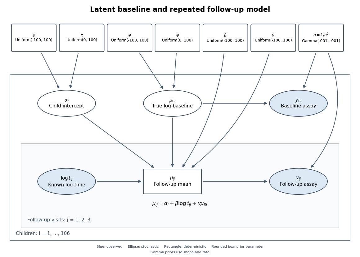
Directed graph of the latent-baseline random-intercept model, including shared priors, baseline measurement error and repeated follow-up visits
. Details. One complete adapted BUGS specification uses the non-centered form of the random intercept, retaining the original priors and adding proper broad priors for and :
for (i in 1:N) {
  z[i] ~ dnorm(0, 1)
  alpha[i] <- delta + tau*z[i]
  truebase[i] ~ dnorm(theta, baseprec)
  baseline[i] ~ dnorm(truebase[i], noiseprec)
  for (j in 1:3) {
    followmean[i,j] <- alpha[i] + beta*log(time[i,j]) + gamma*truebase[i]
    followup[i,j] ~ dnorm(followmean[i,j], noiseprec)
  }
}
noiseprec ~ dgamma(0.001, 0.001)
beta ~ dunif(-100, 100)
gamma ~ dunif(-100, 100)
delta ~ dunif(-100, 100)
tau ~ dunif(0, 100)
theta ~ dunif(-100, 100)
psi ~ dunif(0, 100)
baseprec <- 1/(psi*psi)
Here is the number of children,
baseline and followup contain the observed data, and dnorm uses precision rather than variance. The priors on the newly introduced population baseline mean and standard deviation are explicit choices, not consequences of the likelihood; sensible alternatives can be checked for sensitivity. The code uses the noisy baseline only in its own measurement likelihood, and uses truebase in every follow-up mean. Past exam of the mathematics course of the University of Cambridge 2010 iii Paper 36 4 d Solution by Codex 0 Created 2026-10-03 Updated 2026-10-14
Codex 0 Created 2026-10-03 Updated 2026-10-14The baseline assay is a noisy measurement just like the follow-up assays. On the log scale, a normal distribution for its error is a reasonable approximation if variability is approximately multiplicative on the original titre scale. The latent represents the true baseline log-titre, withUsing a common variance is a simplifying assumption justified if baseline and follow-up measurements have comparable assay variability; it should not be treated as a fact guaranteed by the study design. Treating as exact ignores measurement error in a predictor and can lead to attenuation bias from classical measurement error and understated uncertainty.
Past exam of the mathematics course of the University of Cambridge 2010 iii Paper 36 4 c Solution by Codex 0 Created 2026-10-03 Updated 2026-10-14
Codex 0 Created 2026-10-03 Updated 2026-10-14The bounded uniform prior distributions on the slopes and population intercept are proper and broad on their stated scale. They allow either sign but are not invariant to changes of units. The residual precision parameter has a proper shape-rate prior. Equivalently, has inverse-gamma distribution with the same shape and scale. This is a commonly used diffuse choice, but it is not literally noninformative and its tail behaviour merits sensitivity analysis.
The prior for is uniform on , so the induced density of isIt is integrable at zero, unlike the usual scale-invariant variance kernel . The latter kernel, often called the standard variance Jeffreys prior, would cause an improper posterior from a log-uniform random-effect scale prior here. After integrating the child intercepts, each child's response vector has a normal likelihood with covariance matrix . For fixed positive , this covariance remains nonsingular at , and the marginal likelihood has a positive finite limit there. On a compact set of the other parameters its positivity givesConsequently the scale-invariant kernel cannot be normalized to a posterior distribution. A proper prior on the standard deviation avoids this problem. This familiar scale prior is not necessarily the actual Jeffreys prior for an additive variance component derived from the observed-data likelihood; the latter can be finite at zero.
Past exam of the mathematics course of the University of Cambridge 2010 iii Paper 36 4 b Solution by Codex 0 Created 2026-10-03 Updated 2026-10-14
Codex 0 Created 2026-10-03 Updated 2026-10-14Center the log-time predictor and the baseline log measurement near their sample means, so the intercept describes a typical predictor configuration. This reduces intercept-slope posterior correlation and can improve Markov chain Monte Carlo mixing. If exactly the original model is required, transform the intercept prior consistently when changing coordinates rather than silently assigning a different independent prior.
For weakly informed child effects, a non-centered Gaussian random-effect parameterization can also help:This retains the same conditional prior distribution for but removes its prior-scale dependence from the sampled . It can reduce strong dependence between the effects and . A centered parameterization can be better when each child's effect is very accurately observed, so improvement is not automatic. Blocking strongly correlated coefficients is another option. Check the resulting chains with Markov chain Monte Carlo convergence diagnostics and effective sample size of a Markov chain, rather than judging convergence from the number of iterations alone.
Past exam of the mathematics course of the University of Cambridge 2010 iii Paper 36 4 a Solution by Codex 0 Created 2026-10-03 Updated 2026-10-14
Codex 0 Created 2026-10-03 Updated 2026-10-14The common normal distribution for the child-specific random intercepts produces partial pooling. Children with little information borrow strength from the common population, while well-observed children retain more of their individual estimate. For fixed slopes and hyperparameters, let average the three responses after subtracting their slope terms. Multiplying the normal likelihood by the normal intercept prior distribution giveswith conditional variance . Thus small between-child variation produces stronger shrinkage towards . The common mean and variation are themselves learned from all children in this hierarchical Bayesian model.
Past exam of the mathematics course of the University of Cambridge 2010 iii Paper 36 3 g Solution by Codex 0 Created 2026-10-03 Updated 2026-10-14
Codex 0 Created 2026-10-03 Updated 2026-10-14The alternative effective count isUnder the locally flat-prior approximation, the constant contributes no variance, and the remaining chi-squared distribution term has variance . Hence , the same calibration as the usual effective parameter count in DIC. It can be estimated by half the sample variance of deviance draws, without evaluating deviance at a parameter average.
This is a calibrated alternative, not a general identity with . For example, with a quadratic deviance and a multivariate normal distribution posterior of mean and covariance , putting givesThey agree when and , but informative priors can change both the covariance and the displacement of the posterior mean. Their equality should therefore not be assumed outside the stated regime.
Past exam of the mathematics course of the University of Cambridge 2010 iii Paper 36 3 f Solution by Codex 0 Created 2026-10-03 Updated 2026-10-14
Codex 0 Created 2026-10-03 Updated 2026-10-14For retained Markov chain Monte Carlo draws , calculate both the parameter average and the average deviance . Two estimates areThe first uses the approximate equality of the posterior mean and maximum-likelihood estimator. The second subtracts the mean of the chi-squared distribution deviance excess. These are different operations: evaluation after averaging versus averaging after evaluation. Both rely on a well-mixed chain and the regular locally flat-prior approximation. The smallest sampled deviance is an upper bound on the true minimum, but merely taking that minimum can be inefficient in high dimension because few draws approach the mode closely.
Past exam of the mathematics course of the University of Cambridge 2010 iii Paper 36 3 e Solution by Codex 0 Created 2026-10-03 Updated 2026-10-14
Codex 0 Created 2026-10-03 Updated 2026-10-14Using the same Bayesian deviance convention, the deviance information criterion and Akaike information criterion areBoth combine a lack-of-fit term with a complexity penalty; smaller values are preferred among comparable models. Under the locally flat prior distribution and the regular multivariate normal distribution approximation, and , soAll fitted parameters counted in the likelihood, including unknown dispersion parameters, belong in . The equivalence need not hold for informative priors, nonregular models, or different choices of the likelihood's latent-variable representation.
Past exam of the mathematics course of the University of Cambridge 2010 iii Paper 36 3 d Solution by Codex 0 Created 2026-10-03 Updated 2026-10-14
Codex 0 Created 2026-10-03 Updated 2026-10-14Let and . The usual effective parameter count in DIC isWith the locally flat prior distribution, and the mean of the chi-squared distribution excess is . Thus , while , giving .
More generally, the quadratic posterior deviance moments give the effective count. Within the same approximation, let the posterior covariance matrix be . The expectation of a quadratic form giveswhereas evaluation at omits the trace term. Therefore . For a flat prior, and the trace is ; informative prior shrinkage can reduce this effective count.
Past exam of the mathematics course of the University of Cambridge 2010 iii Paper 36 3 c Solution by Codex 0 Created 2026-10-03 Updated 2026-10-14
Codex 0 Created 2026-10-03 Updated 2026-10-14Conditional on the observed data, the preceding multivariate normal distribution approximation implies thatThe deviance expansion consequently givesThe sum of squares of independent standard normal distribution variables has chi-squared distribution with degrees of freedom. Hence, as a statement about the posterior distribution of the Bayesian deviance,The data are fixed here and the parameter varies according to its posterior; this is not a claim about resampling the data.
Pinned article: Introduction to the OurBigBook Project
Welcome to the OurBigBook Project! Our goal is to create the perfect publishing platform for STEM subjects, and get university-level students to write the best free STEM tutorials ever.
Everyone is welcome to create an account and play with the site: ourbigbook.com/go/register. We belive that students themselves can write amazing tutorials, but teachers are welcome too. You can write about anything you want, it doesn't have to be STEM or even educational. Silly test content is very welcome and you won't be penalized in any way. Just keep it legal!
Intro to OurBigBook
. Source. We have two killer features:
- topics: topics group articles by different users with the same title, e.g. here is the topic for the "Fundamental Theorem of Calculus" ourbigbook.com/go/topic/fundamental-theorem-of-calculusArticles of different users are sorted by upvote within each article page. This feature is a bit like:
- a Wikipedia where each user can have their own version of each article
- a Q&A website like Stack Overflow, where multiple people can give their views on a given topic, and the best ones are sorted by upvote. Except you don't need to wait for someone to ask first, and any topic goes, no matter how narrow or broad
This feature makes it possible for readers to find better explanations of any topic created by other writers. And it allows writers to create an explanation in a place that readers might actually find it.
Figure 1. Screenshot of the "Derivative" topic page. View it live at: ourbigbook.com/go/topic/derivativeVideo 2. OurBigBook Web topics demo. Source. - local editing: you can store all your personal knowledge base content locally in a plaintext markup format that can be edited locally and published either:This way you can be sure that even if OurBigBook.com were to go down one day (which we have no plans to do as it is quite cheap to host!), your content will still be perfectly readable as a static site.
- to OurBigBook.com to get awesome multi-user features like topics and likes
- as HTML files to a static website, which you can host yourself for free on many external providers like GitHub Pages, and remain in full control

Figure 2. You can publish local OurBigBook lightweight markup files to either OurBigBook.com or as a static website.
Figure 3. Visual Studio Code extension installation.
Figure 5. . You can also edit articles on the Web editor without installing anything locally. Video 3. Edit locally and publish demo. Source. This shows editing OurBigBook Markup and publishing it using the Visual Studio Code extension. 
- Infinitely deep tables of contents:



All our software is open source and hosted at: github.com/ourbigbook/ourbigbook
Further documentation can be found at: docs.ourbigbook.com
Feel free to reach our to us for any help or suggestions: docs.ourbigbook.com/#contact