At any $z\ne 0$, take sufficiently small $h$ so $z+h\ne 0$. The complex difference quotient isHence the complex derivative exists at every point of the punctured plane, andThe excluded point is essential to the domain statement: the reciprocal has a simple pole there.

Under the assumed continuous real differentiability, the necessary and sufficient conditions are the Cauchy-Riemann equations at every point of $U$:Necessity follows by computing the complex derivative along real and imaginary increments. For sufficiency, real differentiability gives the first-order expansionThe Cauchy-Riemann equations turn the linear part into $(u_x+i{v}_x)h$, so the complex derivative exists and equals $u_x+i{v}_x$. Thus $f$ is a holomorphic function on $U$.

For the Gaussian integers, use the Gaussian normTo identify the ideal, note that $a^2+b^2$ is even if and only if $a,b$ have the same parity. AlsoThis quotient is a Gaussian integer precisely when $a,b$ have the same parity. Therefore the prescribed set consists exactly of the multiples of $1+i$, givingAny associate of $1+i$ would generate the same principal ideal.

For the zero ideal, choose $d=0$. Otherwise choose a nonzero $d\in I$ for which the Euclidean function $\delta (d)$ is minimal; the well-ordering principle guarantees such a choice. For any $a\in I$, perform Euclidean division:Because $I$ is an ideal, $r=a-qd\in I$. A nonzero remainder would contradict the minimal choice of $d$, so $r=0$ and $a\in Rd$. Thus $I\subseteq Rd$. Conversely, $d\in I$ implies $Rd\subseteq I$, provingEvery ideal is therefore a principal ideal; in particular, a Euclidean domain is a principal ideal domain.

A Euclidean domain is an integral domain $R$ admitting a Euclidean function $\delta :R\setminus \{0\}\to {\mathbb{Z}}_{\ge 0}$ such that division with a smaller remainder is possible: for every $a\in R$ and nonzero $b\in R$, there are $q,r\in R$ withThus the Euclidean function measures progress in repeated division. Definitions which additionally normalize it to be nondecreasing under multiplication give the same class of Euclidean domains; the division property is the one needed below.

First suppose $E=E^{\ast }$. For $u\in U=\mathrm{im}E$, choose $v$ with $Ev=u$. For $w\in W=\ker E$,Thus $U\subseteq W^{\perp }$. The direct sum of vector spaces gives $\dim U=\dim V-\dim W$, while the orthogonal complement has $\dim W^{\perp }=\dim V-\dim W$. Equal finite dimensions imply $U=W^{\perp }$.

Conversely, suppose $U=W^{\perp }$. Decompose arbitrary vectors as $v=u+w$ and $v^{\prime }=u^{\prime }+w^{\prime }$, with $u,u^{\prime }\in U$ and $w,w^{\prime }\in W$. Since $E$ is the indicated projection, $Ev=u$ and $E{v}^{\prime }=u^{\prime }$. Orthogonality makes the cross terms vanish, soTherefore $E$ satisfies the defining identity of its own adjoint operator. By uniqueness from part (a), $E=E^{\ast }$. HenceThis is the characterization of an orthogonal projection among projections along a complementary subspace.

The adjoint operator $T^{\ast }$ is characterized byThis identity works with either convention for which argument of the complex inner product is linear, provided the convention is used consistently.

For uniqueness, subtract the two given identities to get $⟨v,(S-T^{\ast })w⟩=0$ for every $v,w$. Fix $w$ and choose $v=(S-T^{\ast })w$. Then positive definiteness givesso $(S-T^{\ast })w=0$. As $w$ was arbitrary, $\boxed{S=T^{\ast }}$. The decisive fact is that a vector orthogonal to every vector, including itself, must be zero.

Every $g_i\in U^0$ vanishes on $U$, so $U\subseteq {\bigcap }_i\ker g_i$. Conversely, suppose $v\in {\bigcap }_i\ker g_i$. Every $f\in U^0$ is a linear combination ${\sum }_i{a}_i{g}_i$, giving $f(v)=0$. If $v\notin U$, part (b) supplies a functional in $U^0$ with $f(v)\ne 0$, a contradiction. ThereforeFor the dimension statement, take a basis $u_1,\dots ,u_m$ of $U$ and extend it to a basis $u_1,\dots ,u_n$ of $V$. Relative to the corresponding dual basis, a functional belongs to $U^0$ precisely when its first $m$ coefficients are zero. ThusIf $U=V$, this says $k=0$ and the empty intersection is understood to be $V$.

In the coordinate example choose the linear functionals $g_1(x,y,z)=y$ and $g_2(x,y,z)=z$. Their kernels are the two coordinate planesTheir intersection is the stated axis, and $k=2=3-1$.

Choose a basis $u_1,\dots ,u_m$ of $U$. Because $v\notin U$, the list $u_1,\dots ,u_m,v$ is linearly independent. Extend it to a basis of $V$. A linear functional is specified uniquely by its values on a basis, so define $f$ to be zero on the $u_j$ and on every added basis vector other than $v$, and set $f(v)=1$.

Then $f$ vanishes on every linear combination of the $u_j$, so $f\in U^0$, whileThis proves that the annihilator of a vector subspace separates every vector outside the subspace from that subspace; no inner product or preferred coordinates are needed.

The dual space is the vector space of all linear functionals on $V$:Addition and scalar multiplication are defined pointwise. The annihilator of a vector subspace isIt is a vector subspace of $V^{\prime }$: linear combinations of functionals vanishing on $U$ also vanish on $U$.

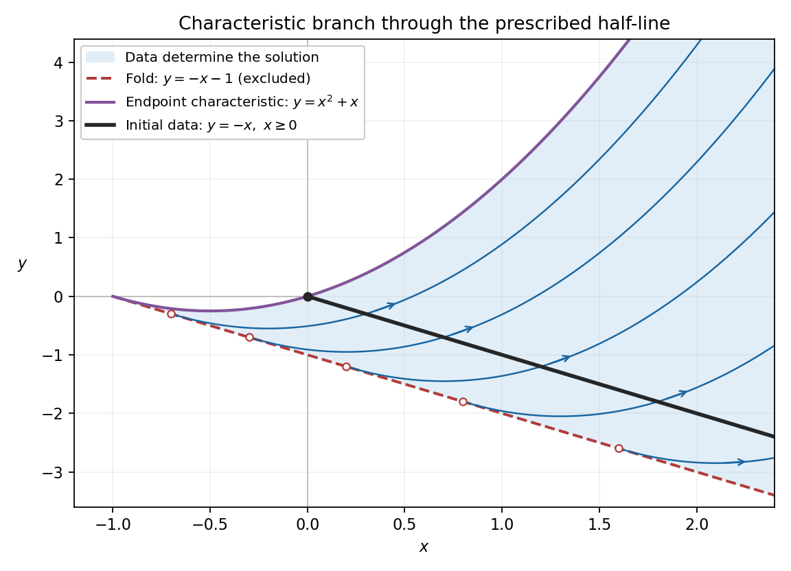
To find the characteristic domain from data on a half-line, retain the allowed range of its initial parameter. The portion connected to the initial data before the fold caustic has $s>-1$ and $t\ge 0$. Inverting the positive branch givesThe square root must be positive, and $t\ge 0$ requires $x+1\ge \sqrt{1+x+y}>0$. Squaring is now legitimate and gives $y\le x^2+x$. Thus the full characteristic-covered set on this branch isIts open interior, where both the data parameter and the projection are interior and nonsingular, is the classical domain of dependence

Each point of $D$ has exactly one backward characteristic meeting the interior $t>0$ of the prescribed data, so the Picard-Lindelöf theorem fixes its value. The upper boundary is the characteristic issuing from the endpoint $t=0$ and is fixed by the endpoint datum, consistently with the continuous trace from $D$. The lower boundary is excluded: $s=-1$ there, the Jacobian determinant vanishes, and the explicit solution derivatives diverge as $W\downarrow 0$.

Points of the half-plane $W>0$ outside this set have $t<0$ on the branch through the data. Their characteristic footpoints would lie on the unprescribed continuation of the initial line, so these values are not determined by the given half-line alone. For example, extend the initial value to negative $t$ as $1+\epsilon h(t)$, where $h$ is a smooth function supported on the negative half-line. Such extensions agree with all the prescribed data and, where noncharacteristic, produce different local extensions by the method of characteristics. The displayed formula supplies one possible extension there, but the data do not select it uniquely. This is why retaining the restriction on the initial half-line is essential. Continuing the parameterized surface past $s=-1$ instead produces the other sheet of the fold; it does not give a differentiable graph continuation through the caustic.

Put $W=1+x+y$. The identity $W=(s+1{)}^2$ gives $s=-1\pm \sqrt{W}$, and hence $z=-1\pm 2\sqrt{W}$. On the initial half-line $W=1$ and the prescribed value is $z=1$, which selects the positive sign. The branch containing the data has $s>-1$, soFor $W>0$, its derivatives are $z_x=z_y=W^{-1/2}$. Substitution checks the partial differential equation:On the data $y=-x$, the value is one. The other algebraic branch gives $z=-3$ there and does not meet these data. The positive-branch formula defines a solution on the larger half-plane $W>0$, but the part uniquely fixed by the prescribed half-line also requires a nonnegative characteristic footpoint $t$, as part (vi) explains.

Differentiating the projected parameterization givesIt vanishes exactly when $s=-1$. The image is the tangency half-line from part (iii), $x=t-1$, $y=-t$, $t\ge 0$. This is a fold caustic: the parameterized surface itself remains regular, but its projection ceases to be locally invertible, so it cannot there be expressed as a differentiable single-valued graph over the plane.

For fixed $t$, eliminate $s=x-t$ to obtain the projected parabolaAlong that curve,Equality occurs at $s=-1$, where the point is $(t-1,-t)$. Also $dy/dx=y_s/x_s=1+2s=-1$ there, so the tangent line has the same slope as the line $x+y=-1$ and passes through a point of that line. Thus every projected characteristic is tangent to that line, with no crossing of it. Because $t\ge 0$, the attained tangency points form only the half-line $x\ge -1$, $y=-x-1$.

Use $t\ge 0$ to label the initial half-line, with $(x,y,z)=(t,-t,1)$ at $s=0$. In the general characteristic from part (i), this sets $a=t$, $b=-t$, $c=1$. The parametric solution surface is thereforeAt $s=0$ this recovers exactly the given data. Moreover $(x_s,y_s,z_s)=(1,1+2s,2)=(1,z,2)$, so the surface follows the required characteristic vector field. The branch defining a classical graph through the data is determined below by restricting to the side of the projection fold containing $s=0$.

The characteristic equations for a quasilinear equation here areSuccessive integration gives the general characteristicwhere $a,b,c$ are integration constants. Equivalently $z-2x$ and $y-z^2/4$ are constant along each curve: differentiating them with respect to $s$ gives zero. Three constants occur because shifting the origin of the parameter $s$ describes the same geometric curve again; there are two independent curve invariants.

An unstable spiral hasRotation is accompanied by exponentially increasing radius in suitable real coordinates. Thus nearby nonconstant orbits spiral away, and the equilibrium is unstable. This is also called an unstable focus.

A stable spiral has the complex conjugate eigenvaluesIn suitable real coordinates the radius decays like $e^{\alpha t}$ while the angle changes at rate $\beta$. The orbit therefore spirals towards the equilibrium, which is asymptotically stable. This is also called a stable focus.

A centre equilibrium of the linearized real planar system hasAfter a real invertible linear change of coordinates, the system is a constant angular rotation. Its nonzero orbits are ellipses of period $2\pi /|\omega |$, so it is stable but not asymptotically stable. This is a classification of the linearization: a centre in the linearization need not be a nonlinear centre. In particular, imaginary eigenvalues alone do not prove a nonlinear centre equilibrium, which requires a punctured neighbourhood filled with periodic orbits. Part (c) illustrates exactly this limitation.

A saddle equilibrium hasThe negative eigenvalue gives a stable manifold direction and the positive eigenvalue an unstable manifold direction. Perturbations along the latter grow, so the equilibrium is unstable even though there are special trajectories approaching it.