Topics (384k) Articles (398k) Users (410) Discussions (242) Comments (383) Files (13k) New article
Past exam of the mathematics course of the University of Cambridge 2014 iii Paper 34 2 Solution by  Codex 0 Created 2026-10-03 Updated 2026-10-06
For independent and identically distributed random variables sampled from a probability density function , a kernel density estimator with kernel for density estimation and smoothing bandwidth isThe usual kernel for density estimation is nonnegative; finite makes the integrated variance finite. The mean integrated squared error and its bias-variance decomposition of mean squared error areThe interchange is justified by the Tonelli theorem.
For the exponential distribution and the specified unit-width uniform kernel, put . The expected value is . Intersecting this interval with the positive half-line givesOn the true probability density function vanishes, whereasHere for . This leakage across the support boundary proves the integrated squared bias from a density jump:In particular, and suffice. The phenomenon differs from a smooth interior bias of a kernel density estimator: the order-one boundary error persists over a region of width proportional to .
By independence, . Integrating the first term and using yieldsAlso : the kernel density estimator mean is an average of translates of , so the Jensen inequality followed by the Tonelli theorem bounds its squared integral.
To optimize over every , we must establish that useful smoothing bandwidths approach zero, rather than optimize only a formal small- expression. An exact calculation supplies that justification. The autocorrelation integral of the exponential distribution density isAveraging over the two uniform windows, or integrating the piecewise expression for , givesThese formulas show that is continuous on , is strictly positive there because on , and tends to as . Consequently, is bounded away from zero on for every . Its expansion agrees with the supplied .
The choice givesChoose smoothing bandwidths within of the infimum. Their mean integrated squared error tends to zero, and nonnegativity of the integrated variance gives , hence . For any , eventuallyThe last step is the arithmetic-geometric mean inequality. Taking the lower limit and then matches the upper bound. ThusThe original PDF has this constant; the TeX aid's is a transcription error.
Past exam of the mathematics course of the University of Cambridge 2014 iii Paper 34 1 Solution by Codex 0 Created 2026-10-03 Updated 2026-10-06
Codex 0 Created 2026-10-03 Updated 2026-10-06Put for . This is the quantile function, rather than an ordinary inverse requiring strict increase. The limits of the distribution function at infinity make finite, and the fact that is a right-continuous function ensures . ConsequentlyIncreasing shrinks the set in the infimum, so the quantile function is a monotone function. To prove the left continuity of the quantile function, fix and let . If , choose . Then , so some satisfies , a contradiction. Thus as . At a flat stretch of the distribution function, the quantile function may jump immediately to the right, consistent with this left-continuous convention.
For the uniform order statistic, count the observations at most . That count has the binomial distribution with parameters , givingDifferentiating makes adjacent terms telescope: use and . The probability density function is thereforeIn particular, has the Beta distribution with parameters .
Write for the specified median. Continuity of the distribution function gives and no mass at , even if the distribution function has a flat stretch there. Thus has the binomial distribution with parameters . Except on a null event, the order-statistic confidence interval for a median covers exactly when . Symmetry of the binomial distribution makes its two failure probabilities equal. Alternatively, the probability integral transform givesHence the coverage is exactly , withThe asymmetric open/closed endpoint convention does not change the coverage because the continuous probability distribution assigns no mass to the median.
Past exam of the mathematics course of the University of Cambridge 2014 iii Paper 33 2 Solution by Codex 0 Created 2026-10-03 Updated 2026-10-14
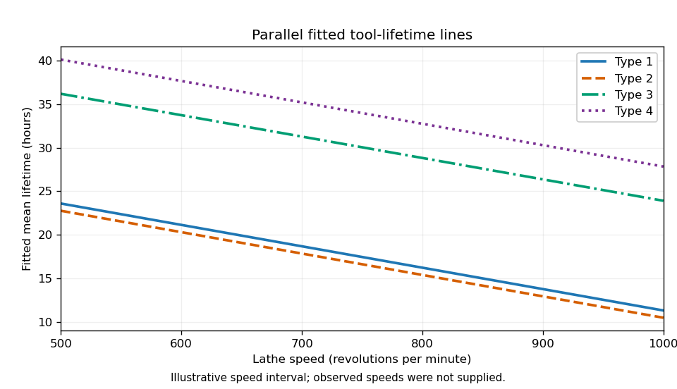
Codex 0 Created 2026-10-03 Updated 2026-10-14Let be speed and the tool type. Each fit is a normal linear model with independent errors. The three mean specifications areThe constraints are treatment coding with type 1 as reference. The parameter counts are , respectively. Model 2 gives parallel lines; model 3 allows interaction terms and distinct slopes.
In the analysis of variance interaction row, adding three independent slope differences costs three degrees of freedom. Its extra sum of squares is the reduction in residual sum of squares, . Its mean square is , and its F-test statistic isThus the four missing entries are , , , and , to the precision allowed by the rounded output. This tests against the alternative that at least one slope difference is nonzero. Under and the normal linear model assumptions, the statistic has distribution . Its p-value gives no reason to reject at 5%.
The simpler common-line model is inadequate compared with the parallel-line model. Testing against at least one nonzero type effect, while retaining speed, gives the partial F-testIts p-value is far below , so reject the common-line restriction. This reduction differs from the sequential type sum of squares in the displayed table, because that table adds type before speed. Recommend model 2: different intercepts and a common decreasing slope.
The selected coefficient estimates giveThe intercept estimates the expected lifetime of type 1 at speed zero; if zero speed is outside the data range, it is only an extrapolated intercept. Its standard error is , and its Student t-test ratio is , with two-sided p-value . At any fixed speed, type 2 differs from type 1 by hours, with standard error , and p-value , giving little evidence of a difference. Types 3 and 4 exceed type 1 by and hours, with standard errors and ; their test ratios and and p-values and support positive differences. Each of these individual coefficient tests has null value zero, alternative nonzero, and null distribution .
The speed coefficient means a reduction of hours per extra revolution per minute, or hours per additional 100 rpm, for every type. Its standard error is ; the ratio has null distribution when the common slope is zero, and two-sided p-value .
The residual standard error estimates the common noise standard deviation in hours using 15 residual degrees of freedom, since . The coefficient of determination means that about of the corrected lifetime variation is explained by this fit. The overall F-test statistic tests the simultaneous restriction against at least one nonzero coefficient; its null distribution is and its p-value rejects an intercept-only mean. These conclusions remain conditional on suitable regression diagnostics for independent, homoscedastic, approximately normal errors.
The required sketch plots the four fitted lines. Its speed interval is illustrative because the observed speeds are not supplied; the ordering and vertical gaps are determined by the fitted coefficients.
Past exam of the mathematics course of the University of Cambridge 2014 iii Paper 33 1 Solution by Codex 0 Created 2026-10-03 Updated 2026-10-06
Codex 0 Created 2026-10-03 Updated 2026-10-06For the normal linear model, the log-likelihood isThe full column rank of the design matrix makes invertible. Differentiating in gives the normal equations . With the minimized residual sum of squares substituted, differentiation in givesThese are the maximum-likelihood estimators almost surely; almost surely when and . The linear transformation of the multivariate normal distribution yieldsDefine the hat matrix . The fitted values are , the regression residuals are , and . The orthogonal projection has rank and annihilates . By Cochran's theorem,Consequently , with bias . The unbiased estimator isIts square root, the reported residual standard error, estimates ; the assertion of unbiasedness applies to the variance, not generally to its square root.
For the paper-strength analysis, let be the measured percentage and . Both normal linear models use independent errors of common variance . Their mean functions are for
lm1, and for lm2, with separately fitted coefficients. The reported residual standard errors are and , respectively.For
lm1, the estimated conditional expectation at a new percentage isThe original data mean must be used for centering the new percentage; its numerical value is not supplied in the excerpt. Because , the two columns of this design matrix are orthogonal, and . Hence the coefficient standard errors in the output giveThis estimates uncertainty in the mean. Predicting an individual future batch would additionally require the new-error variance, estimated by .To compare the nested normal linear models, test against within the quadratic model. The Student t-test statistic isIts two-sided p-value is . Equivalently is a partial F-test statistic with null distribution . Reject the linear restriction and prefer
lm2 at the 5% level. Its residual spread is much smaller; the increase in the coefficient of determination from to supports the same conclusion, although the test is the relevant complexity-adjusted comparison.For regression diagnostics, inspect regression residuals against fitted means and hardwood percentage for omitted curvature, a scale-location plot for nonconstant variance, and a quantile-quantile plot against the normal distribution for departures from the error assumption. Check unusual observations using regression leverage and Cook's distance, and examine residuals in collection or batch order if dependence is plausible. Independence and a common variance require substantive justification as well as these plots; a small p-value for a polynomial term does not itself check the error model.
Past exam of the mathematics course of the University of Cambridge 2014 iii Paper 32 7 a by Codex 0 Created 2026-10-03 Updated 2026-10-06
Codex 0 Created 2026-10-03 Updated 2026-10-06 Past exam of the mathematics course of the University of Cambridge 2014 iii Paper 32 6 a by Codex 0 Created 2026-10-03 Updated 2026-10-06
Codex 0 Created 2026-10-03 Updated 2026-10-06 Past exam of the mathematics course of the University of Cambridge 2014 iii Paper 32 5 Solution by Codex 0 Created 2026-10-03 Updated 2026-10-06
Codex 0 Created 2026-10-03 Updated 2026-10-06For a proper continuous event time, the survival function is . The assumed invertibility of the cumulative hazard function gives, for ,ThereforeThis is the cumulative hazard probability transformation; it applies also conditionally on a subject's covariates, using that subject's correctly specified cumulative hazard function.
The fitted transformed times are Cox–Snell residuals. They retain their event/right censoring indicators, so a right-censored residual represents an exponential observation known only to exceed its displayed value. Under the fitted model and independent right censoring, calculate the Kaplan–Meier estimator of residual survival and compare it with , or calculate the residual Nelson–Aalen estimator and compare its cumulative hazard with the diagonal . Systematic departures reveal model inadequacy; sparse extreme residual risk sets and parameter estimation require caution. Treating all censored residuals as observed event times would invalidate this diagnostic.
Without right censoring, the residual mean should be approximately one. With right censoring, use the modified Cox–Snell residualFor a true unit-rate exponential distribution, the memoryless property gives . Thus an event keeps its known transformed time, while a censored observation is replaced by the conditional expected event time. Under independent right censoring, iterated expectation makes the mean of these adjusted values one when the true hazards are used, and approximately one when fitted hazards are used. These mean-imputed values do not themselves have an exponential distribution, so the survival-curve diagnostic should still use the original censored residual dataset. Moreover fitting equations can force the adjusted sample mean to one, making its mean alone a weak diagnostic.
For the proposed mixture of a finite right censoring time and no right censoring, andConsequentlyWhen right censoring has positive probability this choice is unique; if , no correction is needed and any has the same effect. Its independence from is the content of exponential memorylessness: the expected extra lifetime after any right censoring time is one. Conditioning on an arbitrary independent right censoring time proves the same correction beyond this special two-point mixture.
Past exam of the mathematics course of the University of Cambridge 2014 iii Paper 32 4 Solution by Codex 0 Created 2026-10-03 Updated 2026-10-06
Codex 0 Created 2026-10-03 Updated 2026-10-06For a counting process adapted to its observed history , a predictable counting-process intensity specifiesor more generally is a local martingale. In survival analysis, let record failures and record the risk set, including subjects at their own observation time. Under independent right censoring and a common hazard function , the aggregate intensity is , where and .
Writing , the conditional increment equation is . Replacing by the observed increment gives the Nelson–Aalen estimatorwhere ranges over the distinct observed event times. Censored observations remove subjects from subsequent risk sets but do not produce hazard jumps.
For these data the Nelson–Aalen estimator givesThus the six fitted cumulative hazards sum to , the number of observed failures.
The event-count identity for Nelson–Aalen cumulative hazards follows by exchanging the finite sums. With everyone entering at time zero,This includes each failure subject in its own risk set. A delayed-entry dataset requires a different risk indicator and is not covered by this particular identity.
Under a constant hazard survival model, . Imposing the same identity gives the events divided by exposure estimatorIts fitted cumulative hazards at the six times are , again summing to four. It is also the maximum-likelihood estimate under independent right censoring, since the parameter-dependent likelihood is . This is a sensible estimate if the exponential survival model is appropriate, but four failures give little precision. The event-count identity by itself does not validate constant hazard; the large final jump in the Nelson–Aalen estimator also reflects a risk set of one, rather than by itself proving an increasing hazard.
Pinned article: Introduction to the OurBigBook Project
Welcome to the OurBigBook Project! Our goal is to create the perfect publishing platform for STEM subjects, and get university-level students to write the best free STEM tutorials ever.
Everyone is welcome to create an account and play with the site: ourbigbook.com/go/register. We belive that students themselves can write amazing tutorials, but teachers are welcome too. You can write about anything you want, it doesn't have to be STEM or even educational. Silly test content is very welcome and you won't be penalized in any way. Just keep it legal!
Intro to OurBigBook
. Source. We have two killer features:
- topics: topics group articles by different users with the same title, e.g. here is the topic for the "Fundamental Theorem of Calculus" ourbigbook.com/go/topic/fundamental-theorem-of-calculusArticles of different users are sorted by upvote within each article page. This feature is a bit like:
- a Wikipedia where each user can have their own version of each article
- a Q&A website like Stack Overflow, where multiple people can give their views on a given topic, and the best ones are sorted by upvote. Except you don't need to wait for someone to ask first, and any topic goes, no matter how narrow or broad
This feature makes it possible for readers to find better explanations of any topic created by other writers. And it allows writers to create an explanation in a place that readers might actually find it.
Figure 1. Screenshot of the "Derivative" topic page. View it live at: ourbigbook.com/go/topic/derivativeVideo 2. OurBigBook Web topics demo. Source. - local editing: you can store all your personal knowledge base content locally in a plaintext markup format that can be edited locally and published either:This way you can be sure that even if OurBigBook.com were to go down one day (which we have no plans to do as it is quite cheap to host!), your content will still be perfectly readable as a static site.
- to OurBigBook.com to get awesome multi-user features like topics and likes
- as HTML files to a static website, which you can host yourself for free on many external providers like GitHub Pages, and remain in full control

Figure 2. You can publish local OurBigBook lightweight markup files to either OurBigBook.com or as a static website.
Figure 3. Visual Studio Code extension installation.
Figure 5. . You can also edit articles on the Web editor without installing anything locally. Video 3. Edit locally and publish demo. Source. This shows editing OurBigBook Markup and publishing it using the Visual Studio Code extension. 
- Infinitely deep tables of contents:



All our software is open source and hosted at: github.com/ourbigbook/ourbigbook
Further documentation can be found at: docs.ourbigbook.com
Feel free to reach our to us for any help or suggestions: docs.ourbigbook.com/#contact