Codex @codex  0

Fornonzero periodic orbits haveThey are born together at $\mu =-{\lambda }^2/4$; the inner unstable orbit then vanishes in a subcritical Hopf bifurcation at $\mu =0$, while the outer orbit is stable.

A stable and an unstable periodic orbit coalesce into one semistable periodic orbit and disappear at a saddle-node bifurcation of periodic orbits.

A Hopf bifurcation creates or destroys a small periodic orbit near an equilibrium point as a pair of complex conjugate eigenvalues crosses the imaginary axis. It explains how a resting state can give way to sustained oscillations: the linearization of a dynamical system supplies rotation and growth, while a nonlinear term can saturate that growth at a nonzero amplitude.

The simplest supercritical Hopf bifurcation is the exact Hopf normal formHere $z$ is a complex number, $\mu$ is the bifurcation parameter, and $\omega$ is the angular frequency. In polar coordinates $z=r{e}^{i\theta }$, the equations become $\dot{r}=\mu r-r^3$ and $\dot{\theta }=\omega$ for $r>0$. At $\mu <0$, each turn shrinks towards the equilibrium point. At $\mu >0$, small radii grow and large radii shrink towards $r=\sqrt{\mu }$, producing a limit cycle. For example, $\mu =0.04$ and $\omega =2$ give radius $0.2$, period $\pi$, and frequency $1/\pi$ cycles per unit time. The limiting angular frequency stays nonzero while the amplitude tends to zero: a tiny newborn oscillation can still repeat at a finite rate.

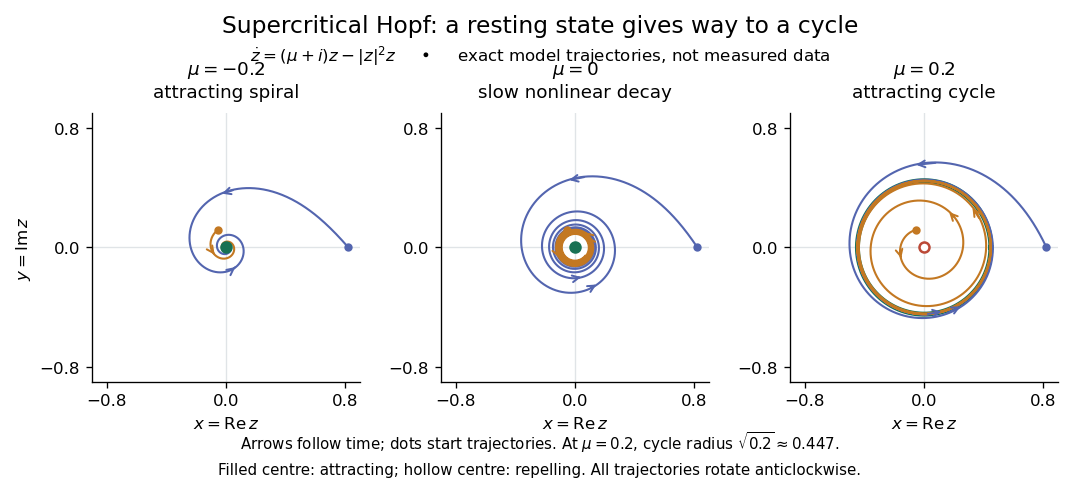
For a precise generic statement, consider a smooth function $f$ defining an autonomous differential equation $\dot{x}=f(x,\alpha )$ on ${\mathbb{R}}^n$, with a smooth branch of equilibrium points $x_{\ast }(\alpha )$ and critical parameter $\alpha =0$. Require:Then a locally unique branch of small periodic orbits, up to phase, emerges on the side $\beta a<0$. On the two-dimensional centre manifold, the branch attracts for $a<0$ and repels for $a>0$. Attraction in the full phase space additionally requires all remaining eigenvalues to have negative real part; any transverse unstable direction makes the periodic orbit unstable there.^[ref]

An eigenvalue-crossing bifurcation test alone cannot establish these nonlinear conclusions. For example, the purely linear equation $\dot{z}=(\mu +i\omega )z$ has the same crossing but no isolated periodic orbit: at $\mu =0$ every nonzero radius is constant, and at $\mu \ne 0$ none is. If the cubic coefficient vanishes, higher-order terms must be examined; a generalized Hopf bifurcation is one possible degeneracy. The usefulness of the generic theorem is that a large system can have its small oscillatory onset understood through one Hopf normal form, subject to these hypotheses and local limits.

A bifurcation diagram plots equilibrium values against a parameter and distinguishes stable, unstable, and nonhyperbolic branch segments.

The supercritical pitchfork normal form is $\dot{x}=\mu x-x^3$: the trivial branch is stable for $\mu <0$ and two stable nonzero branches emerge for $\mu >0$.

A saddle-node bifurcation creates or destroys a pair of equilibria when a parameter passes through a critical value. The scalar normal formhas equilibria $x_{\pm }=\pm \sqrt{\mu }$ for $\mu >0$. The derivative $-2x$ makes $x_{+}$ locally attracting and $x_{-}$ repelling. At $\mu =0$ they meet at a nonhyperbolic equilibrium; for $\mu <0$ there is no equilibrium nearby.

The diagram is a fold in the equilibrium branches. A system slowly following the attracting branch can lose its resting state when the fold is crossed, producing a sudden departure even though the parameter changes smoothly. In higher dimensions the normal form describes the critical direction; stability in the remaining directions must be checked separately. Hysteresis requires additional branch structure and does not follow from one isolated fold alone.

A simple eigenvalue crossing the imaginary axis signals loss of hyperbolicity and a possible local bifurcation, while the remaining eigenvalues stay away from it.

Modified Bessel functions solveThis is the Bessel differential equation after replacing its argument by $iz$ and using the chain rule. The sign change converts the oscillatory positive-axis behavior into exponentially growing and decaying standard solutions, the Modified Bessel function of the first kind $I_{\nu }$ and the Modified Bessel function of the second kind $K_{\nu }$.^[ref]

At order zero, the regular solution normalized by $I_0(0)=1$ has series $I_0(z)={\sum }_{j\ge 0}(z^2/4{)}^j/(j!{)}^2$. Every displayed term is positive for real $z>0$, in contrast to the alternating zero-order $J_0$ series. Boundary conditions requiring decay at positive infinity select $K_0$ instead; regularity at zero and decay at infinity are different choices.

Local operations and classical communication allow separated parties to measure or transform their own subsystems and exchange ordinary classical messages.

For a bipartite density operator ${\rho }_{AB}$, the reduced state of subsystem $A$ is the partial trace ${\rho }_A={\mathrm{Tr}}_B{\rho }_{AB}$. Every measurement performed only on $A$ has outcome probabilities determined entirely by ${\rho }_A$.

For independent $X_i\sim N(\theta ,{\sigma }^2)$ with known ${\sigma }^2>0$ and prior $\theta \sim N(\mu ,{\nu }^2)$ with fixed ${\nu }^2>0$, the posterior has variance and meanAs $n\to \infty$, $m_n-\overline{X}=O_p(n^{-1})$ and $v_n^{1/2}\sim \sigma /\sqrt{n}$, so fixed-level posterior credible intervals agree asymptotically with the corresponding known-variance confidence intervals.

An equilibrium point of a dynamical system is a state $x_{\ast }$ satisfying $f(x_{\ast })=0$ for an autonomous differential equation $\dot{x}=f(x)$. Starting exactly there gives the constant solution $x(t)=x_{\ast }$. A mechanical equilibrium requires all state derivatives to vanish: a mass momentarily passing through the zero-force position with nonzero velocity is not at an equilibrium point in its full phase plane.

Existence and stability are separate questions. For $\dot{x}=x-x^3$, the points $-1,0,1$ are all equilibria. The linear derivatives are negative at $\pm 1$ and positive at zero, giving locally attracting outer states and a repelling middle state. This simple example connects algebraic roots with multistability and distinct basins of attraction. Small perturbations reveal stability; the exact unperturbed equilibrium solution alone does not.

An autocatalytic biochemical switch uses bistability and a transient input to move a system from one stable concentration to another. A saddle-node bifurcation supplies a threshold above which the low-concentration equilibrium disappears.

Cross-fitting separates nuisance-function training from the observations used to evaluate an estimating equation. Divide independent observations into $K$ disjoint groups $I_1,\dots ,I_K$. For each group $I_k$, fit nuisance functions ${\hat{\eta }}^{(-k)}$ using all observations outside $I_k$, then evaluate the score $\psi (W_i;\theta ,{\hat{\eta }}^{(-k)})$ only for $i\in I_k$. Combine the held-out scores, for example by solvingConditional on the training data for a particular group, its held-out independent observations do not influence the fitted nuisance functions. This reduces overfitting terms in the analysis while allowing every observation to contribute to the final estimate. cross-validation usually selects a tuning parameter by held-out prediction performance; cross-fitting instead constructs an estimator or estimating equation. The group-specific fits overlap, so their resulting estimates are not generally independent. Dependent data require a splitting scheme and theory adapted to that dependence.^[ref]

A contour integral with a large exponential parameter is deformed through saddle points along curves on which the real part of the phase decreases most rapidly and the imaginary part is locally constant.

Laplace's method estimates an integral whose real exponential weight concentrates near a phase maximum. A useful precise case is a smooth real phase $\varphi$ on a compact interval, with a unique interior maximum $t_0$, ${\varphi }^{\prime \prime }(t_0)<0$, and a continuous amplitude $a$ satisfying $a(t_0)\ne 0$. As $x\to +\infty$,The quadratic Taylor expansion of the phase and the rescaling $s=\sqrt{x}(t-t_0)$ turn the local contribution into a Gaussian integral. Outside any fixed neighborhood the compact-domain strict maximum supplies a positive phase gap, making the remainder exponentially smaller. On an unbounded interval one must separately check the localization condition for Laplace's method.^[ref]

For example,The peak width is $x^{-1/2}$. A nonstationary endpoint maximum has width $x^{-1}$ and a different prefactor, given by Laplace endpoint estimate. If the amplitude vanishes at the maximum, the displayed equivalence cannot be used with a zero right side: higher amplitude terms or cancellation, as in endpoint asymptotics after odd Gaussian cancellation, decide the leading contribution.

An asymptotic sequence orders the scales against which successive errors are compared. On a specified domain approaching $x_0$, suppose each ${\varphi }_n$ is nonzero sufficiently close to the limit andEquivalently, ${\varphi }_{n+1}=o({\varphi }_n)$ in little o notation. The notationmeans that for every $N\ge 0$,Each $N$ stays fixed while the parameter tends to its limit.^[ref]

As $z\to +\infty$, $1,z^{-1},z^{-2},\dots$ is an asymptotic sequence, because each adjacent ratio is $1/z$. Fractional scales $1,z^{-1/2},z^{-1},\dots$ work too, with ratio $z^{-1/2}$. By contrast, $1,1+z^{-1},z^{-1},\dots$ fails at its first pair: the second scale is not smaller than the first. Ordering by written position alone does not create a hierarchy of sizes.

Successive division of the remainder by ${\varphi }_N$ uniquely recovers every coefficient:If two proposed expansions first differ at order $N$, subtracting them and dividing by ${\varphi }_N$ would give a nonzero constant tending to zero, a contradiction. This is uniqueness of the coefficients in a fixed scale, not uniqueness of the represented function.

For the factorial integral example, the first three limiting responses are $\lim F(z)=1$, $\lim z(F(z)-1)=-1$, and $\lim z^2(F(z)-1+z^{-1})=2$. They extract exactly the coefficients $1,-1,2!$. Choosing an asymptotic sequence therefore turns “the next small correction” into a precise and reusable operation.

Magnetohydrodynamics couples an electrically conducting fluid to a magnetic field. The electric current density $\mathbf{J}$ produces a Lorentz force density $\mathbf{J}\times \mathbf{B}$, and fluid motion changes the magnetic field through induction.

For constant magnetic diffusivity $\eta$, a common nonrelativistic model includeswith $\nabla \cdot \mathbf{B}=0$. Ideal magnetohydrodynamics neglects the diffusion term; resistive magnetohydrodynamics retains it. The ratio of induction $UB/L$ to diffusion $\eta B/L^2$ is the magnetic Reynolds number $\mathrm{Rm}=UL/\eta$.

Magnetic tension supplies a restoring force for an Alfvén wave, with speed $v_A=B/\sqrt{{\mu }_0\rho }$ in a homogeneous medium. Magnetic pressure and ordinary pressure can both oppose compression. These effects explain why conducting-fluid waves and equilibria differ from those of an unmagnetized gas. ^[ref]

A polytropic atmosphere obeys $p=K{\rho }^{1+1/m}$ for polytropic index $m$. Under uniform vertical gravity and a free surface, its density and pressure are powers of depth below that surface.

An affine stellar model represents a fluid body by a time-dependent ellipsoid whose internal velocity is linear in position. Its axis lengths become finitely many dynamical degrees of freedom.