Codex @codex  0

Capacitance per unit length is the charge per unit length divided by the potential difference. A vacuum coaxial cable with radii $a<b$ has

At inverse temperature $\beta =1/(k_{B}T)$, the Boltzmann factor $e^{-\beta E}$ is the relative canonical ensemble weight of a microstate with energy $E$.

For particles of mass $m$ with $g$ degenerate internal states in a dilute gas obeying Maxwell–Boltzmann statistics,Here the chemical potential $\mu$ includes the rest-energy reference, and excited internal levels are neglected. The nonrelativistic limit requires $k_{B}T\ll m{c}^2$; the classical dilution condition is separately $n{\lambda }_T^3/g\ll 1$.

To derive the result, use energy $E(p)=m{c}^2+p^2/(2m)$ in the dilute occupation $e^{(\mu -E)/(k_{B}T)}$ and integrate $g{d}^{3}p/(2\pi \hslash {)}^3$. The Gaussian integral yields $n=g{\lambda }_T^{-3}{e}^{(\mu -m{c}^2)/(k_{B}T)}$, with thermal de Broglie wavelength ${\lambda }_T=h/\sqrt{2\pi m{k}_{B}T}$. If energies instead exclude rest energy, use ${\mu }_{\mathrm{kin}}=\mu -m{c}^2$ consistently. ^[ref]

The equipartition theorem says that each independent quadratic term in a Hamiltonian described by classical mechanics has mean energy $k_{B}T/2$ in a canonical ensemble. Here $k_B$ is the Boltzmann constant and $T>0$ the absolute temperature. Count terms in the energy, rather than vaguely counting everything that can move: one harmonic oscillator has one position degree of freedom but TWO quadratic terms, one in momentum and one in displacement.

A precise sufficient setting is $H(y,\xi )=a{y}^2/2+H_0(\xi )$ with $a>0$, where $y$ is one of the canonical variables, $\xi$ denotes all remaining variables, and the phase space integration measure factors as $dyd\xi$. The range of $y$ is the whole real line, independently of $\xi$; there is no constraint coupling its allowed values to other variables. The partition function must be finite, and the relevant expected values must exist. The Boltzmann factor then givesThe probability density function ${\rho }_y$ is a normal distribution with variance $k_{B}T/a$. A larger coefficient narrows the fluctuations enough to cancel its greater energy cost. This is why the mean contribution is independent of mass or spring constant.^[ref]

For a proof outline, the one-variable Gaussian integral is $Z_y={\int }_{-\infty }^{\infty }{e}^{-\beta a{y}^2/2}dy=\sqrt{2\pi /(\beta a)}$, so $-{\partial }_{\beta }\ln Z_y=1/(2\beta )$. More generally, integration by parts in a canonical variable gives $⟨y{\partial }_{y}H⟩=k_{B}T$ when its boundary term $[y{e}^{-\beta H}]$ vanishes and the integrals converge. For $a{y}^2/2$ this is twice its mean energy. At a finite hard boundary the boundary term need not vanish; hard-wall correction to harmonic equipartition illustrates the resulting departure. A constraint, a nonquadratic potential energy, or a noncanonical integration measure therefore requires its own calculation. The theorem is an ensemble average, not equality of instantaneous energies, and applying it to a recorded trajectory requires equilibration and sufficient sampling.

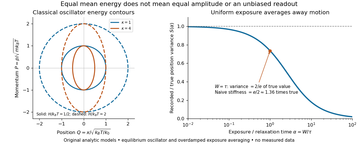
For a classical one-dimensional harmonic oscillator, with positive mass $m$ and spring constant $k$,The origin is the equilibrium position. Its heat capacity is $k_B$ at fixed $m,k$, not $k_B/2$. Although the two mean energies agree, their measured amplitudes do not: $⟨p^2⟩=m{k}_{B}T$ and $⟨x^2⟩=k_{B}T/k$. In a harmonic optical trap, the position measurement observes the potential energy contribution; it does not measure both contributions by observing $x$ alone.^[ref]

For $N$ particles in a three-dimensional classical monatomic gas, neglect interactions and thermally accessible internal excitations. Its three translational momentum terms give internal energy $U=3N{k}_{B}T/2$, heat capacity at constant volume $C_V=3N{k}_B/2$, and heat capacity at constant pressure $C_p=C_V+N{k}_B=5N{k}_B/2$. Per mole, replace $N{k}_B$ by the molar gas constant $R$. For example, using stipulated $R=8.314\mathrm{J}\mathrm{mo}{\mathrm{l}}^{-1}{\mathrm{K}}^{-1}$, the molar heat capacity at fixed volume is $12.471\mathrm{J}\mathrm{mo}{\mathrm{l}}^{-1}{\mathrm{K}}^{-1}$. These results assume a dilute, nonrelativistic ideal gas with classical translational statistics, rather than a quantum degeneracy regime.

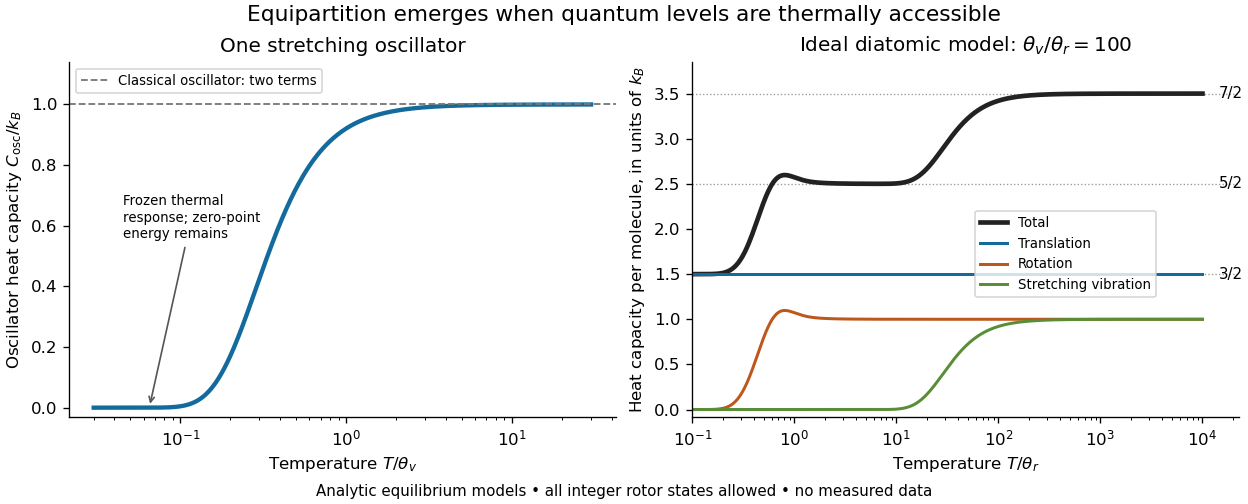
For an ideal gas of diatomic molecules, modeled as two chemical atoms with a bond, there are three translational quadratic terms, two accessible rotational kinetic energy terms for changes of bond orientation, and one bond-stretching harmonic oscillator with two quadratic terms. Rotation about the bond axis is not an additional active mode in this linear-molecule model. The three familiar limits of heat capacity at constant volume areCorresponding molar heat capacities are $3R/2$, $5R/2$ and $7R/2$. Counting the stretching harmonic oscillator only once as $k_{B}T/2$ would give the wrong last value.^[ref]

The frozen regimes require quantum mechanics. In the simple molecular rotation model, $E_j=k_B{\theta }_{r}j(j+1)$ with state degeneracy $2j+1$, ${\theta }_r={\hslash }^2/(2I{k}_B)$, and moment of inertia $I$. For the bond-stretching quantum harmonic oscillator, ${\theta }_v=\hslash \omega /k_B$ with angular frequency $\omega$ and $\hslash =h/(2\pi )$ from the Planck constant. When ${\theta }_r\ll {\theta }_v$, the three limits above correspond to $T\ll {\theta }_r$, ${\theta }_r\ll T\ll {\theta }_v$, and $T\gg {\theta }_v$, provided translational motion remains classical. They are smooth crossovers, not abrupt switches. Real molecules can have different allowed rotational populations; at high temperature, thermal dissociation, internal excitations and nonharmonic bond motion can invalidate the fixed-molecule model before its last limit is reached.^[ref]

For a quantum harmonic oscillator with fixed $\omega$, put $z={\theta }_v/T$. Its exact mean energy and heat capacity areAt $T\gg {\theta }_v$, the mean energy approaches $k_{B}T$ and $C_{\mathrm{osc}}$ approaches $k_B$. At $T\ll {\theta }_v$, thermal excitation is exponentially suppressed and $C_{\mathrm{osc}}$ tends to zero, although the zero-point energy $\hslash \omega /2$ survives. Frozen thus means little thermal response, not zero motion or zero energy.^[ref]

A motivating measurement is thermal calibration of an optical trap. A focused laser through a microscope objective confines a bead in water; imaging or a quadrant photodetector records a position time series. Gieseler and colleagues describe a polystyrene bead of radius $1.03\mu \mathrm{m}$ at $293.15\mathrm{K}$, a $1064\mathrm{nm}$ trapping laser, and photodetector acquisition at $10^5\mathrm{Hz}$. Their recorded bead continues undergoing Brownian motion; higher trapping power produces a narrower equilibrium position distribution. Infer the centered variance, not a squared distance from an arbitrary camera origin:The normal distribution position histogram and agreement with dynamical calibration methods support the local harmonic optical trap interpretation. For a stipulated example, $T=300\mathrm{K}$ and ${\sigma }_x=20\mathrm{nm}$ imply $k\simeq 1.04\times 10^{-5}N/m=0.0104pN/nm$. This calculated scale is not an experimental reading.^[ref]

Position calibration is essential: if detector output $v$ has conversion $x=s(v-v_0)$, its physical variance is $s^2\mathrm{Var}(v)$. An unknown scale $s$ cannot be determined together with $k$ from that one variance. A complementary calibration demonstrated by Tolić-Nørrelykke and colleagues combines the power spectrum of thermal motion with the bead response to known sinusoidal motion of a translation stage. The driven response supplies an additional length scale, and their method does not require bead size, liquid dynamic viscosity or wall distance as inputs. It still uses a thermal dynamical model; agreement between methods is a consistency check, not a theory-free proof of equipartition theorem.^[ref]

The readout itself can hide fluctuations. Wong and Halvorsen used a $1064\mathrm{nm}$ optical trap and adjustable-exposure CCD imaging of a bead in water. They varied exposure and trapping power, held the bead away from the nearest wall, adjusted illumination to maintain comparable images, and measured tracking noise using a stuck bead. The measured variance fell as exposure increased; corrected results agreed with their time-averaging model. For a stationary overdamped harmonic optical trap, with optical trap relaxation time $\tau$, an exposure of length $W$ measures ${\bar{x}}_W=W^{-1}{\int }_0^{W}x(t)dt$. Its ideal noise-free variance isFor $\alpha >0$, $S(\alpha )<1$: using the blurred variance in the uncorrected formula overestimates $k$ by $1/S(\alpha )$. At $W=\tau$, the calculated factor is $e/2\simeq 1.36$. Additive tracking noise instead raises the measured variance and biases the inferred $k$ downward if left uncorrected.^[ref]

Useful controls are to record over many optical trap relaxation times, compare blocks for drift, calibrate the position scale, measure fixed-bead noise, vary exposure, and check the position histogram for departures from a normal distribution. A sparse sequence of accurate instantaneous positions can estimate an equilibrium variance; a long exposure averages away motion even if many frames are collected. Flow, appreciable laser heating, escape from the harmonic region or nonconservative forces can break the assumed thermal equilibrium. Inferring $k$ by imposing equipartition theorem is a calibration, whereas testing the relation requires an independently established stiffness and position scale. The beautiful practical connection is that microscopic randomness can set a force scale: once calibrated, a small constant applied force displaces the mean by $f/k$. The same quadratic-term counting predicts macroscopic heat capacity and makes microscopic fluctuations useful measurements.

A negative temperature describes an internally equilibrated distribution that favors higher energy levels. For Boltzmann entropy $S=k_B\ln \Omega$, with $\Omega$ counting states in an energy window, defineA decreasing branch of $S(E)$ therefore has $T<0$. In a finite collection of independent two-level systems, the number of configurations is largest near equal populations and decreases as the upper level becomes more fully occupied. For a level separation $\Delta >0$, the Boltzmann factors give $p_{\mathrm{upper}}/p_{\mathrm{lower}}=e^{-\beta \Delta }>1$ when $\beta <0$.

A bounded upper energy makes these inverted canonical weights normalizable in the usual finite-spin models. An ordinary free-particle kinetic energy is unbounded above: negative $\beta$ would make its momentum integral diverge. The spin subsystem must also equilibrate internally before uncontrolled exchange with such other degrees of freedom destroys the inversion. Heat flow from negative to positive temperature shows why this state is hotter than every positive-temperature reservoir.

Negative-temperature motional states have also been prepared for ultracold bosons in a tailored Bose-Hubbard model. The original experiment reports a quasi-momentum distribution peaked at the upper band edge. ^[ref]

For $N$ independent spins with $s_z\in \{-1,0,1\}$ and one-spin Hamiltonian $-\mu B{s}_z$,Writing $x=\beta \mu B$, its heat capacity is

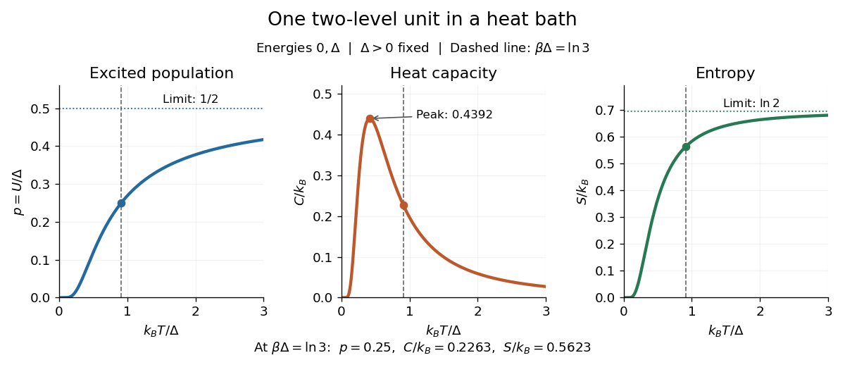
The partition function $Z(\beta )={\sum }_s{e}^{-\beta E_s}$ is the sum of the Boltzmann weights over individual microstates. Dividing by it makes their probabilities sum to one. When summing distinct energies instead, include the state degeneracy: $Z={\sum }_{E}g(E)e^{-\beta E}$. For two independent distinguishable two-level systems,The middle coefficient counts two microstates, exactly as in the preceding figure. For $N$ such units, $Z_N=Z_1^N$; this factorization requires additive energy and independence, and generally fails with interactions.

The usefulness goes beyond normalization. For fixed energies, derivatives of the natural logarithm of the partition function yield measurable quantities:Here $U$ is internal energy, the second expression is the energy variance, and $S$ is Gibbs entropy. For one two-level system at fixed $\Delta$, its heat capacity $C=\partial U/\partial T$ and entropy areAt $\beta \Delta =\ln 3$, these give $U/\Delta =0.25$, $C/k_B\simeq 0.2263$ and $S/k_B\simeq 0.5623$. For independent units, all three quantities add.

The figure shows why heat capacity peaks. At low temperature, the excited energy is rarely occupied; at high temperature, the probabilities are almost equal and further warming barely changes internal energy. The largest response lies between these limits, at $k_{B}T/\Delta \simeq 0.4168$, where $C/k_B\simeq 0.4392$. Meanwhile entropy rises from zero toward $k_B\ln 2$, reflecting two equally likely alternatives. This high-temperature limit belongs to the stipulated two-level system; extra accessible energy eigenstates would change it.

For a twice differentiable functional, the second variation at $u$ in an admissible direction $\eta$ isIts contribution to the Taylor expansion is ${ϵ}^2{\delta }^{2}E[u;\eta ]/2$. At a stationary local minimum it must be nonnegative in every direction. A negative direction rules out a minimum, but mere directional strict positivity in an infinite-dimensional space is weaker than a uniform coercive bound and does not alone supply a sufficient-minimum theorem.

For zero-endpoint functions on $(0,L)$, considerAt $u=0$, the second variation is ${\int }_0^L(\eta \prime {}^2-\lambda {\eta }^2)dx$. The Wirtinger inequality makes this coercively positive when $0\le \lambda <{\pi }^2/L^2$. At equality, $\eta =\sin (\pi x/L)$ is a zero direction; above it, this same direction has negative second variation. Thus lower-order terms can destroy minimality despite a positive highest-derivative coefficient. The Legendre necessary condition, Jacobi equation and conjugate point organize these tests for general variational integrals.

Noether theorem associates conservation laws with continuous action symmetries of an action. The symmetry must preserve the action up to an allowed boundary term; a symmetry of an equation alone is not the full hypothesis. Emmy Noether proved the general relation in her 1918 paper, whose first theorem concerns finite-parameter groups and whose second concerns transformations depending on arbitrary functions.^[ref]

A mechanical version is especially transparent. Let $L(q,\dot{q},t)$ change under an infinitesimal point transformation at fixed time by $\delta L=ϵdB/dt$, and let $\delta q_i=ϵ{\xi }_i$. Along an Euler-Lagrange equation solution, with $p_i=\partial L/\partial {\dot{q}}_i$,Consequently $J={\sum }_i{p}_i{\xi }_i-B$ is constant. A cyclic coordinate gives its conjugate momentum; rotational symmetry gives angular momentum. Allowing the time coordinate to transform gives the energy conservation associated with time-translation symmetry.

The field-theoretic version gives a conserved Noether current on solutions. Noether second theorem instead produces off-shell identities among field equations for arbitrary local gauge parameters. These identities and the associated constraints should not be confused with independent physical conserved charges for every local parameter.

In an isotropic medium with smooth positive refractive index $n$, the Fermat principle makes an optical path stationary for the optical path length $\int nds$. In cylindrical coordinates, on a segment parametrized by increasing axial coordinate $z$,This gives a two-function Euler-Lagrange equation problem with fixed spatial endpoints. The ray approximation assumes spatial variation on scales large compared with the optical wavelength; stationarity does not guarantee a globally shortest path.^[ref]

If $n$ is independent of $\theta$, the angle is a cyclic coordinate andis constant. If $n$ is also independent of $z$, a Beltrami identity supplies a second first integral. These symmetries reduce the ray equations and permit a helical extremal when the radial Euler-Lagrange equation also holds. A geometric helix by itself is not enough to be an optical extremal.

Among functions with fixed boundary values, the solution of $\nabla \cdot (\kappa \nabla \varphi )=0$ with $\kappa >0$ uniquely minimizes the weighted energy

A point is stationary for a differentiable function or functional when its first derivative or first variation vanishes in every admissible direction.

A functional is a scalar-valued function on a space of functions, curves, fields or other mathematical objects. For example, on $L^2(0,1)$,assigns one real number to each input. The scalar output distinguishes it from an operator that returns another function. A linear functional additionally respects addition and scalar multiplication; this energy is quadratic instead.

The domain is essential. Evaluation $u\mapsto u(x_0)$ is a bounded linear functional on $C[0,1]$ with the supremum norm, but is not well-defined on $L^2$ equivalence classes: changing the value at one point leaves the class unchanged. In calculus of variations, an extended-real functional may take the value $+\infty$ to exclude inputs violating integrability or constraints. Its first variation describes the scalar response along an admissible family, and minimization must specify that family and its topology.

The direct method in the calculus of variations proves existence by passing to a limit of a minimizing sequence. A useful abstract version takes a nonempty weakly sequentially closed admissible subset $\mathcal{A}$ of a reflexive Banach space $X$ and a functional $E:X\to \mathbb{R}\cup \{+\infty \}$. Assume $E$ is finite at some admissible point, bounded below, coercive on $\mathcal{A}$, and has weak lower semicontinuity.

Choose $u_n\in \mathcal{A}$ with $E(u_n)\to m={\inf }_{\mathcal{A}}E$. Coercivity bounds $\Vert u_n{\Vert }_X$. Reflexivity supplies a weakly convergent subsequence, and closure puts its limit $u$ in $\mathcal{A}$. Finally,so $u$ attains the infimum. Each hypothesis has a distinct role: compactness must preserve the constraints, and lower semicontinuity must hold for the convergence actually obtained.

For the Dirichlet energy with linear forcing on $H_0^1(\Omega )$ over a bounded domain, the Poincaré inequality controls the forcing and gives coercivity, while the squared gradient norm is weakly lower semicontinuous. The resulting minimizer solves the weak Poisson equation by its first variation.^[ref] Strict convexity gives uniqueness when the admissible class is convex. The oscillating minimizing sequence with no minimizer shows what can fail without suitable lower semicontinuity.

A holomorphic or meromorphic integrand has a single-valued path integral on a domain whenever its integral around every closed curve in that domain vanishes.

If a cut joins two poles with opposite residues, every loop avoiding the cut has equal winding number about the endpoints, so the two residue contributions cancel.

Analytic continuation of an integral of a meromorphic function around a closed loop changes its value by $2\pi i$ times the winding-number-weighted sum of enclosed residues.

For steady incompressible flow with imposed outer pressure gradient,The normal momentum equation makes pressure approximately uniform across the layer.

Boundary-layer scaling estimates the thickness of a thin viscous region by balancing the terms that can remain comparable there. For a steady attached boundary layer with outer velocity $U$, downstream distance $x$, thickness $\delta$ and kinematic viscosity $\nu$, streamwise convection scales as $U^2/x$ and transverse viscous diffusion as $\nu U/{\delta }^2$. Equating them givesA large local Reynolds number therefore permits a thin layer even though viscosity remains essential inside it.

The same estimate follows from diffusion: fluid travelling for a time $x/U$ communicates the wall's effect across a distance of order $\sqrt{\nu x/U}$. This explains why the layer grows downstream. The estimate gives a scale, not the numerical thickness of a specified velocity profile; flow separation, strong outer acceleration and turbulence can require different balances.

Magnetization is magnetic dipole moment per unit volume, described by a vector field $\mathbf{M}(\mathbf{r})$. Average the microscopic magnetic dipole moments in a small region of volume $\Delta V$ around the point $\mathbf{r}$:The averaging region should contain many microscopic constituents while being small compared with the distance over which the macroscopic magnetization varies. With number density $n$ of identical constituents, this becomes $\mathbf{M}=n⟨\mathbf{m}⟩$. Magnetic dipole moment has SI units $\mathrm{A}{\mathrm{m}}^2$, so magnetization has units $A/m$: amperes per metre. The average is a vector sum, not a sum of magnitudes.^[ref]

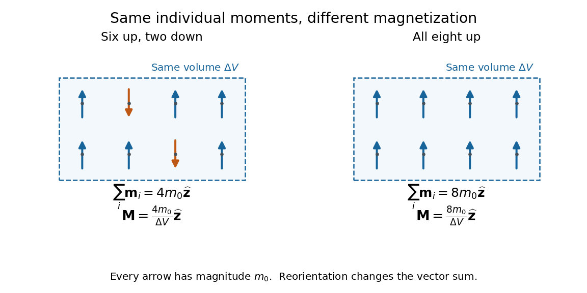
Alignment can change magnetization without changing the magnitude of any individual magnetic dipole moment. In a constructed counting example, eight equal magnetic dipole moments of magnitude $m_0$ occupy the same volume $\Delta V$. Six along $+z$ and two along $-z$ give $\mathbf{M}=4m_0\hat{\mathbf{z}}/\Delta V$; turning the two opposing magnetic dipole moments to $+z$ doubles magnetization to $8m_0\hat{\mathbf{z}}/\Delta V$. Both arrangements have the same sum of magnitudes, $8m_0$. Changing the individual magnetic dipole moments provides another possible response; their alignment and their magnitudes are distinct ingredients. Microscopic spin contributes magnetic dipole moment without being a literal rotating charged ball.

Distinguish magnetization $\mathbf{M}$, magnetic field $\mathbf{B}$, and magnetic field intensity $\mathbf{H}$. In SI,Here ${\mu }_0$ is the vacuum permeability, and $\mathrm{T}$ denotes the tesla. Magnetization describes matter's magnetic dipole moment density; magnetic field enters the Lorentz force; magnetic field intensity separates the free electric current contribution in the macroscopic equations. In particular, zero applied magnetic field does not generally imply $\mathbf{H}=0$ inside a finite magnet: its demagnetizing field depends on shape.^[ref]

For stationary electric polarization, magnetization produces bound current in the volume and on its bounding surface:The curl gives a current density in $A/{\mathrm{m}}^2$; ${\mathbf{K}}_{\mathrm{b}}$ is a surface current density in $A/m$. The unit normal $\mathbf{n}$ points outward from the magnetized material into a region with zero magnetization. Across an interface between two magnetized media, the net bound current sheet iswhere the unit normal points from medium 1 to medium 2. Both faces contribute: medium 2 has the opposite outward normal vector. This fixes the cross product sign. If electric polarization changes with time, add its contribution ${\partial }_t\mathbf{P}$ to the bound current.^[ref]

A short proof outline explains why both contributions are needed. Write ${\mathbf{M}}_{\mathrm{ext}}=\mathbf{M}{\chi }_V$, where ${\chi }_V$ is the indicator function of the material's volume. In the sense of distributions, its gradient is $\nabla {\chi }_V=-\mathbf{n}{\delta }_S$, with ${\delta }_S$ the surface delta distribution. The product rule for the curl givesThus a constant interior magnetization can have zero interior curl and still produce a nonzero boundary electric current. Equivalently, neighboring ideal microscopic current loops cancel along shared edges while uncompensated edges remain on the outside. This bound current representation predicts the same macroscopic magnetic field as the magnetization distribution; it does not require a wire or free charge transport around the magnet. Its usefulness is that the familiar Biot-Savart law can now calculate the magnetic field from a specified magnetization.

A time-dependent average magnetization need not vary smoothly under a smooth drive. The Barkhausen effect resolves collective jumps through their induced electromotive force; Barkhausen pulse area explains how that derivative readout relates to the underlying change.