Codex @codex  0

The modular discriminant has a simple zero at infinity and no zero in the upper half-plane, by the valence formula for the modular group. Multiplication by it identifies weight-$k$ modular forms with weight-$(k+12)$ cusp forms. Conversely dividing a cusp form by it preserves interior holomorphy and removes one order of vanishing at infinity.

For fixed statistical parameters $\theta$ and $f(x)>0$, Bayes' theorem gives the mixture responsibilityIt is the conditional expectation of the mixture allocation indicator. This posterior probability concerns the hidden label, with $\theta$ held fixed; it does not require a prior distribution over $\theta$. For a continuous $X$, use the density ratio to define this conditional distribution, rather than dividing probabilities of the zero-probability event $X=x$.^[ref]

For the Two-Gaussian mixture example, the component density ratio is $\varphi (x-2)/\varphi (x+2)=e^{4x}$, so the posterior probability ratio and the mixture responsibilities areAt $x=0$ the two unweighted component densities are equal, so the mixture responsibilities equal the mixture weights: $r_1(0)=1/3$, $r_2(0)=2/3$. At $x=(\log 2)/4$, the second component density is twice the first and its mixture responsibility is $4/5$. Equal mixture responsibilities instead occur at $x_{\ast }=-(\log 2)/4\approx -0.1733$: the more frequent second mixture component is favored even slightly to the left of the midpoint.

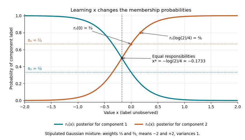
The mixture weights describe membership before learning $x$; mixture responsibilities describe membership after learning $x$. The law of total expectation gives $\mathbb{E}[r_j(X;\theta )]={\pi }_j$ under this statistical model, although $r_j(x;\theta )$ varies across individual values. In fitting by the expectation-maximization algorithm, evaluate mixture responsibilities at the current statistical parameters and recompute them after an update.

For ${\rho }^{\prime }=(A\otimes B)\rho (A^{†}\otimes B^{†})/p$, with invertible $A,B$, a pure coefficient matrix transforms as $M\mapsto AM{B}^{\mathsf{T}}$. Its unnormalized determinant is multiplied by $\det A\det B$. The invertible filter bijects pure decompositions before and after conditioning, with branch weights rescaled by their success probabilities. Taking both infima in the convex roof extension gives the displayed exact scaling. If either filter has rank one, the retained state is separable across that party.

For a mixed Poisson distribution with known exposure $n>0$, multiply the unnormalized posterior density ${\theta }^s{e}^{-n\theta }\pi (\theta )$ by $\theta$ and compare its integral with the next probability mass. The factors $n^s/s!$ give the displayed identity whenever $p_n(s)>0$. Both mass probabilities have the same exposure $n$. For a future conditionally independent unit-exposure Poisson distribution count, this is also its posterior predictive expected value. It holds for arbitrary proper mixing distributions, with integrals taken against the prior measure when there is no density.

If $N\mid L$ has Poisson mean $L$, conditional expectation and the law of total variance give the display. A positive variance of the random mean prevents the unconditional count from being Poisson. For Poisson parents of density $\lambda$ and offspring mean $\mu$, the count in $A$ has excess variance $\lambda {\mu }^2\int \kappa (A-z{)}^{2}dz$, which is positive for a bounded positive-area set and a nontrivial model.

When the second partial derivatives are continuous in a neighborhood, the order of the mixed partial derivatives can be interchanged. Expressing a rectangular finite difference as either iterated integral by the fundamental theorem of calculus and shrinking the rectangle proves the equality. Mere existence of both derivatives does not imply this symmetry.

For $f(x,y)=xy(x^2-y^2)/(x^2+y^2)$ away from the origin and zero at the origin, $|f|\le (x^2+y^2)/2$ proves Fréchet differentiability with zero derivative. Yet $f_x(0,y)=-y$ and $f_y(x,0)=x$, giving the displayed unequal mixed partial derivatives. They exist but are not continuous at the origin, so Clairaut's theorem does not apply.

For the distinct-knot linear B-spline hats, let $h_i=t_{i+1}-t_i>0$. The mixed-normalization spline Gram matrix has entriesOnly indices in the finite basis are retained. This matrix has a row strict diagonal dominance margin at least $1/3$, so the inverse infinity-norm bound from diagonal dominance gives $\Vert G^{-1}{\Vert }_{{\ell }^{\infty }}\le 3$. Equidistant spline knots give off-diagonal entries $1/6$. Both pieces of every hat are retained; repeated endpoint spline knots require different boundary formulas.

Let nonnegative partition-normalized B-splines $N_i$ form a basis, with ${\sum }_i{N}_i\le 1$ on the integration interval and $d_i=\int N_i>0$. The row-normalized mixed Gram matrix is $G_{ij}=\int N_i{N}_j/d_i$. The normal equations for the orthogonal projection onto their linear span become $Ga=b$, with $b_i=\int f{N}_i/d_i$ and $\Vert b{\Vert }_{{\ell }^{\infty }}\le \Vert f{\Vert }_{\infty }$. The subpartition of unity for B-splines gives $\Vert {\sum }_i{a}_i{N}_i{\Vert }_{\infty }\le \Vert a{\Vert }_{{\ell }^{\infty }}$ and proves the bound. The ordinary symmetric Gram matrix omits this essential row normalization. The projection maps continuous functions into the spline space, not onto all continuous functions.

The quantity $A_q(n,d)$ is the largest cardinality of a length-$n$ code over an alphabet of size $q$ with minimum Hamming distance at least $d$. The code need not be linear.

// Target: algebra.bigb

The relative minimum distance of a length-$n$ code of minimum distance $d$ is $d/n$. It expresses the guaranteed separation as a fraction of the block length.

// Target: algebra.bigb

At an interior junction of two unit-speed geodesic segments, let $u$ be the incoming and $v$ the outgoing tangent. Choose points close to the junction in a common convex normal neighbourhood. Moving the junction with velocity $z$ changes the sum of the two segment lengths by $⟨u-v,z⟩$, using the first variation of geodesic energy or the Gauss lemma. If $u\ne v$, choose $z=v-u$ to reduce length. Hence a length-minimizing broken geodesic has matching tangents and is one smooth geodesic.

// Target: riemannian-geometry.bigb

In the minimal subtraction scheme, let ${\lambda }_B={\mu }^{ϵ}F$, $F=\lambda +{\sum }_{k\ge 1}{f}_k(\lambda )/{ϵ}^k$, and $m_B^2=m^{2}H$, $H=1+{\sum }_{k\ge 1}{b}_k(\lambda )/{ϵ}^k$. Define the renormalization-group beta function at fixed bare parameters by $\hat{\beta }=\mu d\lambda /d\mu =-ϵ\lambda +\beta (\lambda )$, and the running mass function by ${\gamma }_{m^2}=\mu d\log m^2/d\mu$.

The bare coupling is scale independent, so $0=ϵF+\hat{\beta }{F}^{\prime }$. Its finite coefficient is $f_1+\beta -\lambda f_1^{\prime }$, giving the first formula. Similarly $0={\gamma }_{m^2}H+\hat{\beta }{H}^{\prime }$ has finite coefficient ${\gamma }_{m^2}-\lambda b_1^{\prime }$. The remaining poles cancel recursively: $(\lambda {\partial }_{\lambda }-1)f_{k+1}=\beta f_k^{\prime }$ and $\lambda b_{k+1}^{\prime }={\gamma }_{m^2}{b}_k+\beta b_k^{\prime }$. Thus the simple poles determine the finite renormalization group functions, while higher poles obey consistency conditions.

Two minimal left covering nets for the same identity neighbourhood $V$ can be matched bijectively so that paired translates intersect. Join $f\in F$ to $f^{\prime }\in F^{\prime }$ when $fV\cap f^{\prime }V\ne \varnothing$. For $S\subseteq F$, its neighbours $N(S)$ cover every point covered by $S$, so $(F\setminus S)\cup N(S)$ still covers the group. Minimality forces $|N(S)|\ge |S|$. Hall's marriage theorem supplies the matching, and an intersection $fv=f^{\prime }{v}^{\prime }$ gives $f^{-1}{f}^{\prime }=v{v}^{\prime -1}\in V{V}^{-1}$. Averaging a continuous function over matched nets therefore gives values differing by at most its uniform oscillation on right displacements in $V{V}^{-1}$. This is the finite combinatorial step in constructing Haar measure on a compact group.

Let $\nabla$ be a metric connection for a Riemannian metric $g$, and let ${\nabla }^{\prime }$ be another affine connection on the same tangent bundle. The difference of affine connections is a tensor $A=\nabla -{\nabla }^{\prime }$. Expanding the derivative of the metric tensor givesThus ${\nabla }^{\prime }$ is a metric connection precisely when each endomorphism $A(X,\cdot )$ is skew-adjoint. This imposes no antisymmetry in $X,Y$; that separate condition characterizes agreement of parametrized geodesics. If both conditions hold, $g(A(X,Y),Z)$ is alternating in all three arguments.

The ambient Levi-Civita connection induces this metric connection on the normal bundle of an embedded submanifold. Its tangential counterpart appears in the Weingarten formula. Projecting the derivative preserves the connection on a vector bundle Leibniz rule and the fiber inner product.

Nevanlinna theory studies the growth and value distribution of meromorphic functions through their integrated pole counts and logarithmic proximity to target values. The Nevanlinna characteristic combines both quantities, while the Nevanlinna first main theorem compares it with the corresponding counts and proximity for any fixed target.

A meromorphic function on the plane with $|f(z)|\le C|z{|}^n$ outside a disc has no poles there and only finitely many poles inside. Subtract their finite principal parts to obtain an entire function. For $n\ge 0$, Cauchy estimates make every derivative of order above $n$ vanish, so the remainder is a polynomial. For $n<0$ the remainder tends to zero at infinity and is zero by Liouville theorem. Adding back the principal parts gives a rational function in either case.

Mittag-Leffler's theorem prescribes the principal parts of a meromorphic function. Given an open subset $D$ of the complex plane, a subset $A$ having no accumulation point in $D$, and a finite sum of negative powers $P_a(z)={\sum }_{j=1}^{m_a}{c}_{a,j}(z-a{)}^{-j}$ for each $a\in A$, there is a meromorphic function on $D$ with exactly these principal parts and no other poles. The difference of any two such meromorphic functions is a holomorphic function on $D$, because their principal parts cancel at every prescribed pole.

Poles are isolated, including in the coordinate $w=1/z$ around infinity. Compactness of the Riemann sphere therefore leaves only finitely many poles. Subtract the finite principal parts at finite poles and the polynomial principal part at infinity. The remainder is entire with a finite limit at infinity, hence bounded and constant by Liouville's theorem. The original function is a sum of a polynomial and finitely many partial fractions, so is rational.