
The scalar potential is . Minimizing it with respect to givesChoose a gauge with constant condensate phase and take the homogeneous-amplitude London limit, . Then c reduces toThe London screening with an unnormalized complex condensate has a factor of two from the complex-field kinetic term as printed; no has been included in the definition of the real positive . Equivalently, the gauge mass is .
For a planar surface at and conductor in , take a tangential field . The solution bounded at large depth isThe exponentially growing solution is excluded. The screening current is nonzero near the surface, demonstrating the Meissner effect through a persistent surface current. The constant-amplitude approximation describes London screening away from any region where the condensate itself is strongly suppressed.
In the stipulated static gauge, . Where this equilibrium screening current is nonzero, the assumed local Ohm's law therefore demands . The simultaneous equality deep in the bulk would by itself place no constraint on ; it is not a valid standalone proof of superconductivity.
The lossless condensate also supplies the dynamical check. With fixed amplitude and phase in temporal gauge, differentiating the London relation gives . A steady field accelerates the supercurrent rather than producing a stationary dissipative current. Thus the ideal condensate has zero electrical resistivity, or an infinite electrical conductivity, consistent with the static screening solution. This is the superconducting component of the toy model; normal carriers and dissipation are not included. The nonzero field expectation is understood in a gauge-fixed description of the Higgs phase, not as a gauge-invariant local observable.
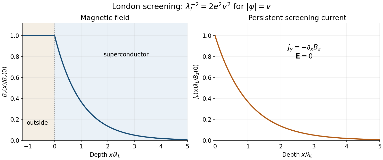
Exponential magnetic screening and the persistent surface current
. Original London-limit half-space solution. The magnetic field and screening-current magnitude share the decay length lambda L; their boundary values set the plotted normalization. Details.Keep the index convention of b: , so and the spatial gauge covariant derivative is . The physical three-current is the spatial part of :Equivalently, writing gives . Under the gauge transformation in a, and , so this expression is manifestly invariant. Switching to a convention with the opposite spatial gauge sign reverses the phase-gradient term, not the screening term proportional to .
For static fields the spatial Ampère-Maxwell equation is , while . Taking its curl yields the general magnetic-field equationNo uniform-condensate approximation has yet been used. For a varying scalar amplitude the gradient terms must be kept; simply replacing by a constant before deriving the current would conceal their origin. The homogeneous-condensate limit supplies the London screening equation in d.
Use and define the physical electromagnetic source by . For a constant infinitesimal phase , the matter Noether current isA definition using phase parameter instead divides this expression by ; the Maxwell source includes the electric coupling shown here. Current signs must be tied to the printed convention.
To verify the equation of motion, vary the matter kinetic term with respect to :Varying and integrating by parts gives . The stationary action therefore requiresThe potential has no explicit dependence on and contributes no extra source term. Antisymmetry of implies on the equations of motion; the same conservation law follows from the scalar equations. The source current is gauge-invariant although its expanded derivative and vector-potential pieces are not separately invariant.[ref]
Quantum Field Theory by David Tong. §§6.1.1 and 6.3.2, gauge symmetry and scalar coupling; the sign here follows the source's minus-sign covariant derivative
The continuous internal symmetry is local gauge invariance. With the source's gauge covariant derivative convention it acts asso transforms like and is unchanged. Constant phases are its global subgroup, not an additional independent internal rotation group.
In flat four-dimensional space-time the continuous external symmetry is the Poincaré group: four translations and six Lorentz transformations. Noether's theorem associates translations with conserved energy and momentum, spatial rotations with angular momentum, and boosts with the relativistic center-of-energy/boost charges. In tensor notation the latter two are the six components of the conserved total angular-momentum tensor , including field spin contributions where appropriate. The nonzero dimensionful parameter prevents exact scale invariance. Discrete transformations, such as parity, are outside the requested continuous-symmetry list.
On the unbounded line the momentum density of states in a reference length is . Count both signs of , each with zero-point energy and the same frequency regulator:The extensive divergent term agrees exactly with c. Subtract it before taking the cutoff away:The force tending to change the interval length isIts negative sign means attraction: separating the boundaries increases this negative vacuum-energy difference toward zero. The bulk subtraction must be made before interpreting the force, otherwise differentiating an unphysical cutoff-dependent bulk energy would contaminate it.
This is the one-dimensional scalar Dirichlet Casimir force. The source's name “Casimir-Polder” normally refers to a retarded atom–atom or atom–surface dispersion force, whose geometry and power law differ. No atom polarizability or electromagnetic mode multiplicity enters the scalar result derived here.
For , the frequencies are . The stipulated spectral regulator therefore supplies . With ,The sum identity follows by differentiating the convergent geometric series with . Its small- expansion issoIn the frequency-regulated Dirichlet Casimir energy, the inverse-length scale suppresses modes with frequency much above in units . It is an ultraviolet cutoff, removed after comparing the same underlying vacuum convention in the two geometries. Physically an ideal perfectly reflecting boundary also ceases to be adequate at sufficiently high frequency, but that material scale is not specified here. The source calls this heat-kernel regularization; its explicit regulator is exponential in frequency, rather than the alternative exponential in frequency squared.
The Hamiltonian density is . In the vacuum only contributes. HenceSubstitution, using , yieldsThis Dirichlet scalar vacuum energy density illustrates why a massive field's local unregularized energy density need not be uniform. The cosine integrates to zero over the interval, soThese divergent expressions are understood with a common regulator before exchanging sums, integrals or derivatives. Normal ordering the Hamiltonian operator separately in each geometry would erase the vacuum terms one is trying to compare; a common regulated subtraction is used instead in c and d.
Separate the Klein-Gordon equation as . The spatial equation is , with . The first Dirichlet boundary condition removes the cosine solution, and the second requires . ThusThere is no nonzero Dirichlet mode. The real field is built from both complex-conjugate time dependences, with mode functionsThe sine functions satisfy . Consequently the factor gives unit Klein-Gordon inner product for each positive-frequency mode and the canonical equal-time field commutator after quantization. A general solution is a superposition of these modes, rather than a claim that a single mode exhausts all solutions.
The leading decay is into one complex particle and its antiparticle, which are distinguishable. Using in a givesIn four space-time dimensions a canonically normalized scalar has mass dimension one, so has mass dimension one. The amplitude starts at order , a rate is quadratic in that amplitude, and the only mass scale in the massless-daughter decay is . Those facts already require , leaving only a dimensionless numerical factor to calculate.
For low-energy charged-scalar scattering through a neutral scalar, label the incoming particle and antiparticle as and their outgoing counterparts as . Charge flow allows -channel annihilation and exchange of the real massive scalar. It forbids a separate -channel graph for this fixed assignment of distinguishable final charges. The tree amplitude isAt low energy it is approximately angle independent. The massless two-body scattering formula then givesIn particular the requested scale estimate is , not with the incoming-energy dependence omitted. Integrating out gives at this order, whose complex-scalar four-leg combinatorics reproduce the same amplitude. These are weak-coupling perturbative results about the specified vacuum; possible ultraviolet stabilizing interactions are not determined by the cubic term alone.
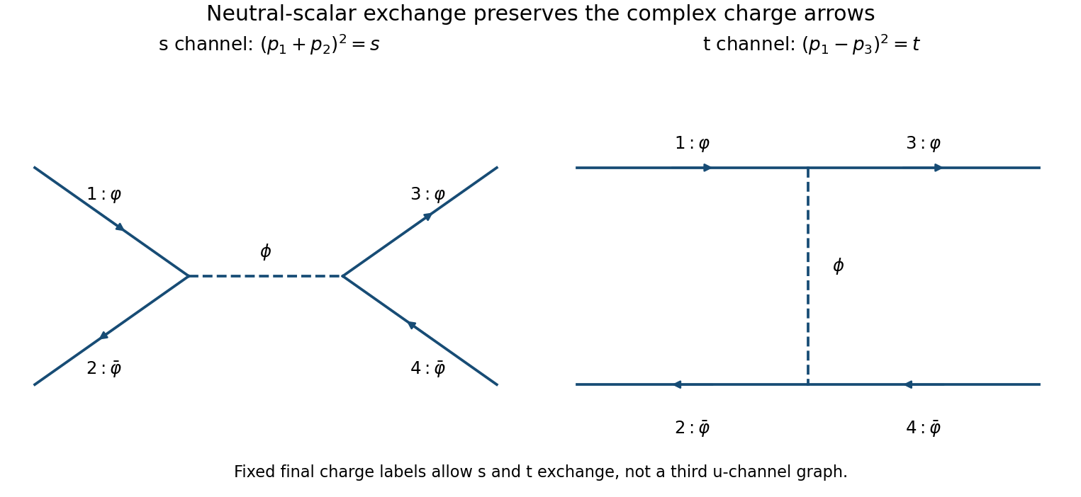
The two allowed leading particle-antiparticle scattering diagrams
. Original s-channel annihilation and t-channel exchange graphs. The internal dashed line is the massive neutral scalar; solid arrows show conserved complex charge. A u-channel graph would connect the wrong final charges for the fixed labeling. Details.At a single interaction insertion, the Dyson series supplies . Amputating the three external propagators in b gives the momentum-space ruleIf the momentum-conservation factor is included in the vertex convention, append , with all momenta incoming. There is one charged line entering and one leaving the vertex, and a neutral real-scalar line. The absence of a factorial in the interaction is appropriate because its three fields are distinct. The amputated decay amplitude has magnitude with the usual convention that a graph computes .
Define the free Feynman propagators byThe interaction preserves the global phase symmetry , with the real neutral. Therefore the charge-two correlator vanishes in a symmetry-invariant perturbative vacuum:In Wick contractions, a complex field contracts only with its conjugate; one vertex has one of each and cannot absorb both external fields. The symmetry shows this vanishing holds to all perturbative orders, not only first order.
The neutral connected correlator has one allowed contraction to each external point at order :The propagators are even functions of their separation; their orientations encode the conjugate-field contractions. Equivalently, with every external momentum Fourier transformed as incoming,No factor of two accompanies the vertex: and are distinct fields.
For the full correlator as literally written, a disconnected scalar three-point tadpole is also possible. Contract the two external complex fields with each other and contract the complex pair at the vertex into a loop. Unless normal ordering is imposed on the interaction or a tadpole counterterm fixes , addThe coincident propagator is regulator dependent; in dimensional regularization the massless scaleless tadpole diagram vanishes. More generally this is to this order and is removed by taking the connected correlator or imposing the stated vacuum-renormalization condition. Normalizing by vacuum bubbles alone does not remove an external-leg disconnected tadpole diagram. The charged correlator remains zero in every one of these conventions.[ref]
Quantum Field Theory by David Tong. §§3.3.2 and 3.7.1, Wick expansion, connected Green functions and vacuum normalization
Evaluate the two-body Lorentz-invariant phase space in the decaying particle's rest frame, . The spatial delta function sets . Both massless particles have energy , leavingHere the factor in the second equality is the Jacobian of the energy delta function. Integrating the solid angle gives . If the decay is isotropic, the squared amplitude is angle independent, soThis uses distinguishable final particles or an amplitude/phase-space convention with any required identical-particle symmetry factor already included. Two genuinely identical final bosons require an additional if the full angular domain is integrated without such a factor. The complex particle and antiparticle in the following parts are distinct, so no such division is required there.
A real antisymmetric generator of the connected rotation group isChoose . Under and , the gauge covariant derivative transforms in the same way as the field. Include the canonical gauge kinetic term so the vector's mass normalization is specified.
In unitary gauge, . The relevant Lagrangian density isReading the quadratic vector term as givesThe angular scalar supplies the longitudinal polarization of the massive vector; it is not a separate physical massless particle after gauging. The physical scalar still has .
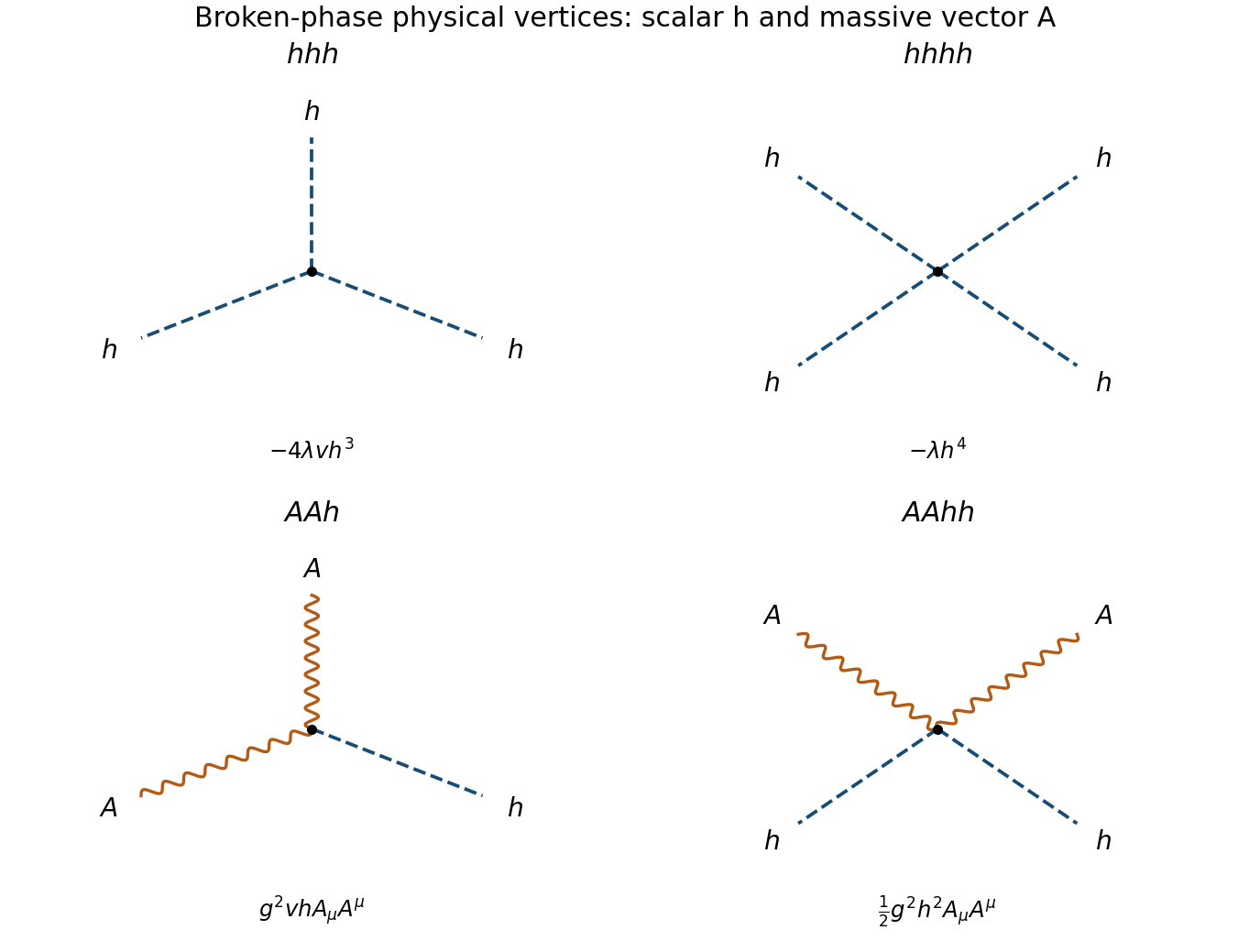
The interactions among the physical fields areThus the complete physical vertex list is , , , and . An Abelian gauge kinetic term generates no or self-interaction. Gauge-dependent Goldstone vertices in another gauge do not add physical particle species to this list. These statements concern the broken phase ; when the unitary-gauge broken-phase parametrization is unavailable.


At an arbitrary nonzero vacuum write , where . The Hessian matrix of the potential isOn the vacuum circle this reduces toIt has eigenvalue along and eigenvalue zero along the one perpendicular direction. Rotating the vacuum conjugates this matrix by an orthogonal matrix and cannot change its eigenvalues. Thus every point on the circle has exactly one tangential massless Goldstone boson.
Geometrically, motion along the circle costs no potential energy whereas motion normal to it does. The circle's dimension, equivalently , is independent of its point. Counting the number of real field components would instead give two and would incorrectly count the massive radial direction as a Goldstone mode.
Any constant real orthogonal matrix acting by preserves both the Euclidean field-space norm and the kinetic term. The full internal symmetry is , with connected component ; reflections add a discrete component.
For , the vacuum manifold is the circle . Expand about the chosen point as , . The potential becomesThe kinetic terms remain canonically normalized real-scalar kinetic terms. Comparing the quadratic potential with givesThere is one massive radial mode and one massless tangential Goldstone boson. A chosen vacuum leaves only the reflection that fixes that point, so there is one broken continuous generator. For negative the chosen point lies on the opposite side of the same circle and the mass depends on ; the radius is . If , the vacuum circle collapses to the origin, no continuous generator is broken, and both quadratic masses vanish without either field being a Goldstone mode. The nonzero- assumption is essential to the spontaneous-breaking interpretation.
With the Minkowski metric , the momentum conjugate to the real field vector is . The Hamiltonian density isAssume the potential has a global minimum and the boundary conditions permit a constant minimizing field. ThenThe bound is attained byThe homogeneous vacuum minimum criterion proves existence of a homogeneous lowest-energy configuration under those assumptions. On infinite space one subtracts the constant vacuum energy before comparing finite energy differences. This identifies the classical vacuum configuration; it does not assert that the quantum field has no fluctuations.
The claim does not follow from “no derivative dependence in ” alone. For example, the allowed functional form is unbounded below, so there is no state of lowest energy to identify. Boundary conditions forcing different vacua at opposite ends can instead require an inhomogeneous minimum, such as a domain wall. The positive quartic potential used in the following parts does have homogeneous minima, so these caveats do not obstruct its vacuum calculation.
At a global reversal leaves the energy and statistical weight unchanged but changes the sign of the one-spin observable. Pairing reversed configurations givesEquivalently, in the transfer eigenbasis, so . This holds for every finite even ring and all finite temperatures, and for the zero-field Gibbs limit. A symmetry-selected zero-temperature alternating state can have nonzero staggered magnetization; its uniform magnetization is still zero. The classical spin variable in this model has no separate quantum spin-operator dynamics despite the conventional matrix notation used for the insertion.
At zero field the normalized transfer matrix for a classical spin chain eigenvectors and eigenvalues areThe spin insertion exchanges the two eigenvectors: and conversely. Evaluating the trace in c therefore gives, with ,This is the finite-ring result. In the thermodynamic limit, or for away from the wrap-around image, it becomesHere is in lattice-site units. The alternating sign is antiferromagnetic order at short distances; the exponential envelope shows the absence of long-range order at every positive temperature in this one-dimensional finite-range model. As , diverges, asymptotically . For the even ring the zero-temperature result is , consistent with the two alternating ground configurations. At fixed finite , “large distance” must still respect periodicity: rather than decaying indefinitely beyond the ring.
Insert the two observed spins into the configuration sum for the transfer matrix for a classical spin chain trace. Since the diagonal matrix has entry on state , multiplication by it at positions and produces the factor . The trace representation is consequentlyThere are exactly transfer factors: . The distance between the two insertions is bonds, not . Cyclicity of the trace combines the outside factors and gives the equivalent expressionwhich makes independence of the starting site manifest. No assumption that commutes with is used; in general it does not. For the two insertions multiply to the identity and , a useful normalization check.
Share each on-site field energy equally between its two neighboring bonds. In the ordered basis , the symmetric transfer matrix for a classical spin chain isThe product recovers each bond and each field term once. Summing the periodic indices closes a trace, giving . The two eigenvalues areThe square-root argument is positive. Moreover , so even at nonzero field. Its sign must not be discarded merely because all matrix entries are positive. The Perron–Frobenius theorem ensures that the positive eigenvalue has the larger modulus, and the infinite-chain free energy is . For even , both terms in the finite-size partition function are positive.
There are unlisted articles, also show them or only show them.