
A massless eigenvector must lie in the null space of , so its coefficients satisfy and . Hence they are proportional to . The original gauge kinetic terms have the Euclidean unit matrix in species space, so normalize this vector by its ordinary squared length. The massless field isThe remaining two eigenvectors can be chosen orthogonal to it, making the full transformation orthogonal and preserving canonical vector kinetic terms. At , the formula is exactly as required. This null direction and its normalization are unaffected by the common mass-scale correction in part b.
For , the massless mode has geometrically unequal components; a matter field coupled to one end can therefore couple more weakly to this surviving vector than a field coupled to the other end. This follows directly from the eigenvector coefficients, without changing the equal microscopic gauge coupling .
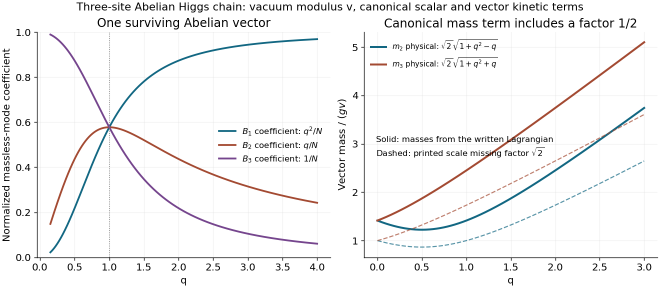
For this three-site Abelian Higgs chain, the potential is minimized by . Choose their phases real in a local unitary gauge. The scalar kinetic terms then givewhere Lorentz contractions are understood andThe nonzero eigenvalues of equal those ofnamely and . The third eigenvalue is zero because has rank two. Both nonzero eigenvalues are positive for .
Mass-normalization correction: the canonical vector mass term is , so the Lagrangian actually gives . Its physical masses are thereforeThe printed dimensionless eigenvalue pattern is correct, but its common scale must be , not , for the written kinetic terms and vacuum value. For a concrete counterexample set and . This is a canonically normalized eigenmode and its mass term is , giving physical squared mass rather than the printed . The printed scale would require a vacuum modulus or a corresponding change in scalar normalization, neither of which is the specified potential minimum.
The unbroken transformations preserve both vacuum phases:Thus the local breaking pattern isTwo scalar phases supply the longitudinal polarizations of the two massive vector bosons; one massless vector remains. This is the Higgs mechanism, with its mass matrix fixed by the scalar charge matrix and the vacuum normalization.[ref]
Gauge Theory by David Tong. Section 2.5.2, expanding scalar kinetic terms around a condensate to obtain a vector mass
Introduce three independent local parameters . A consistent convention for the three Abelian gauge transformations isIndeed, shifts by , cancelling the derivative of the scalar phase. Thus transforms by the same phase as . The two kinetic terms, the absolute-value potentials and all Abelian field strengths are invariant.
In units where the gauge coupling is , the charge vectors under the three factors areLocally this is the gauge algebra of . To interpret it globally as three compact circle groups, the charges must belong to a compatible charge lattice: in the stated unit-charge convention integer is sufficient, while arbitrary irrational is not a single-valued compact-group representation. The local transformations and mass calculation remain meaningful for general positive real as a Lie-algebra calculation, or with noncompact Abelian factors.
For longitudinal-vector annihilation through a scalar contact interaction, first use the supplied vertex . Let and work in the center-of-mass frame. The amplitude is , up to its overall phase. For two longitudinal incoming vectors,This grows as , whereas transverse amplitudes stay of order and mixed longitudinal-transverse amplitudes vanish in this frame. Consequently the leading high-energy contribution is longitudinal.
For an unpolarized total cross section, average over the incoming polarizations. The massive-vector polarization sum givesThe identical final scalars require a factor in the two-body phase space. With and , the angle-independent result isFor a prepared longitudinal pair there is no incoming polarization average, giving insteadThere is no extra initial-state factor : a cross section uses the incoming beam flux, while the final-state factor removes double counting of indistinguishable outgoing states.
Define the energy in the stated bound to be the total center-of-mass energy, . Equating the leading expressions to givesfor and . The second value shows that a longitudinal channel reaches the supplied perturbative bound earlier. If the source's unspecified denotes the energy of one incoming particle and the bound is literally , substitute instead: the corresponding values are unpolarized and longitudinal. Stating the energy and polarization conventions is necessary for a numerical answer.
Interaction-normalization qualification: the written differentiates to , because there are vector assignments and scalar assignments. For example, differentiating twice in each variable gives . The supplied would instead follow from . Thus all cross sections above follow the explicitly requested rule. Using the literal written interaction multiplies them by four and divides every quoted threshold energy by . The energy growth itself is the physical issue: a contact interaction of massive longitudinal vectors needs additional dynamics before its perturbative high-energy extrapolation becomes reliable.
Take with . A real orthonormal basis that satisfies the source's stated bilinear normalization isEach obeys . The two transverse norms are , while , and all cross products vanish. For momentum in the opposite direction, one consistent longitudinal choice is for ; an overall sign of any polarization is immaterial.
Here and label the two linear transverse basis vectors. If those symbols are intended to denote circular helicities, choose instead. The corresponding orthonormality relation must contain complex conjugation, . Without that conjugation, a circular polarization has , a concrete counterexample to interpreting the printed bilinear condition as a helicity normalization.
Varying the vector field gives the Proca equation,Its divergence uses antisymmetry of to cancel the first term. Since ,For an on-shell momentum this imposes on the four polarization components, leaving three independent solutions. In the rest frame, makes , leaving precisely the three spatial polarizations of a massive spin-one particle.
There is no fourth independent oscillator hidden in . Its canonical momentum is zero because the Lagrangian has no , and the temporal equation constrains in terms of the spatial data. Equivalently the primary and secondary second-class constraints remove two variables from the eight-dimensional phase space, leaving six phase-space variables, or three physical degrees of freedom.
The Proca action is invariant under spacetime translations and proper continuous Lorentz transformations, together forming the connected Poincaré group. The fixed nonzero mass excludes scale invariance. In four dimensions, a dimensionless action and the canonical kinetic term implyThese are mass dimensions. The field-strength term is invariant under , but the mass term is not: its change contains . Thus the displayed massive-vector theory has no Maxwell-type local gauge invariance. The massless limit has a different constraint structure.
Choose the current convention corresponding to . Noether's theorem givesFor the requested terms with no and , the Lagrangian is and the current becomes . The supplied covariant oscillator normalization cancels the invariant measure when the annihilation operator contracts with , soThe momentum is on the massless shell, . Differentiating once more therefore givesThis Goldstone current matrix element in a phase-only scalar theory shows that a conserved current can have a nonzero matrix element proportional to a null momentum. Thus current conservation is fully consistent with the current creating a massless one-particle state from the vacuum; the nonzero coefficient is its Goldstone-current coupling. It is the divergence that vanishes, not the current matrix element. Reversing the current convention reverses the nonzero matrix element but leaves this zero divergence unchanged.
Put . Direct differentiation of cancels the mixed radial-angular terms, leavingUse from part b to expand the potential. The complete local expression isThe radial field is canonically normalized, giving . For arbitrary , the canonically normalized angular field is and has zero mass:The interactions comprise radial cubic and quartic self-couplings, a derivative coupling and a derivative coupling. In canonical variables the latter coefficients are and respectively. The additive constant shifts the vacuum energy and does not affect these masses or interactions.
The original phase symmetry becomes the exact shift , with unchanged. Any undifferentiated polynomial or would violate this shift, so such terms are absent. This argument allows derivative interactions; it forbids an angular potential. The massless angular excitation is the Goldstone boson for the broken global .
The scalar potential is . Completing the square givesThe Hamiltonian density also contains the nonnegative terms . Its lowest-energy configurations therefore have no time or spatial variation and minimize the displayed square. ThusThe minima form a circle of phases. Selecting the real positive representative chooses one vacuum and spontaneously breaks the continuous global symmetry in field theory. The stationarity at is a local maximum of the radial potential, not the ground state.
The continuous internal global symmetry in field theory isBoth and are unchanged. The group is the circle group, acting by phase rotations. The ordinary derivatives do not make it a local gauge symmetry: spacetime-dependent would add derivative terms. There is also the discrete symmetry of complex conjugation; in the two-real-field description the full internal invariance is , whose connected component is this .
The rates in part d turn the generating-function equation intoFor the distribution of a critical linear birth-death population, the method of characteristics gives and . Setting gives , so the initial characteristic coordinate is . HenceIt has the correct initial value and . With , rewrite the denominator as and expand its geometric series. The probabilities areAt this is understood by continuity: and all other probabilities vanish. Summing the positive-state probabilities gives , which together with verifies normalization directly.
There is eventual extinction with probability one, because . Nevertheless at every finite time, while . There is no contradiction: the increasingly rare surviving populations have conditional mean . This is the distinction between a constant ensemble mean and survival of a typical realization.
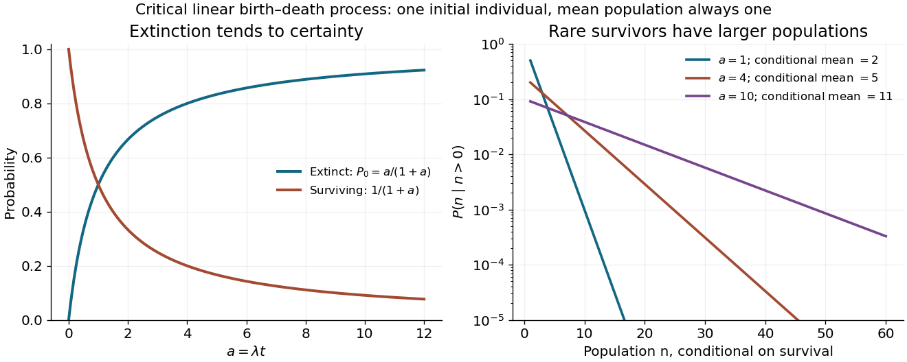
With individuals, each of the can reproduce at rate and independently die at rate . Thus the total birth and death rates are . The gain into state comes from a birth in state and a death in state , while its loss rate is . ThereforeAt , the birth inflow from negative states is absent and . The empty state is absorbing: once the population reaches zero, neither process can restart it. Equal birth and death rates make this a critical branching process.
For the Poisson process, and , soThis is an ordinary differential equation in time for each fixed , with solutionConsequentlyThe initial condition is interpreted as , with all other initial probabilities zero. Normalization follows from . The mean and variance are both , as expected for independent events arriving at constant rate.
Multiply the master equation by and sum over . Shifting indices producesThe apparent negative power causes no problem at when . Let , so . If the rates are polynomials in , replace their arguments by to obtain a finite-order partial differential equation:For arbitrary rates the weighted sums still give an exact generating-function evolution, but need not reduce to a finite-order differential operator. The probability generating function obeyswhich is the normalization condition. The evolution has when the rate sums converge, so an initially normalized distribution stays normalized. Its derivatives at also give the factorial moments, and expansion around recovers individual probabilities.
This is a birth-death master equation: is the transition rate and is the transition rate . The first two terms are incoming probability flows from the adjacent states; the last removes probability at the total escape rate . Rates must be nonnegative. For a population on the nonnegative integers, take and no incoming flux from negative states.
Summing over all states and shifting the two incoming indices givesThus an initially normalized probability distribution remains normalized. The cancellation assumes no boundary flux and legitimate summation; on an infinite state space this means the nonexplosive process or a boundary prescription that conserves total probability. All rates used in the later parts satisfy this requirement.
For nonzero field, the spin-wave ground state is the vacuum of all . The inverse Bogoliubov transformation gives and vanishing one-point oscillator averages. Translational invariance therefore gives the depletionRotating back to the physical axes yields, to the retained spin-wave order,The zero transverse components also follow from rotation by about the physical axis in a symmetry-preserving ground state. The nonzero depletion describes zero-point quantum fluctuations: the original boson vacuum is not the ground state because the anomalous terms create pairs. It is nonnegative and must satisfy for the expansion to be reliable. At strong field it tends to zero, with in the infinite-chain limit.
For fixed , the momentum sum has a finite thermodynamic limit obtained by . At zero field the uniform mode already has no oscillator vacuum, as explained in part d. Even after removing that mode, the nonzero modes behave asThus assigning a finite ordered moment by simply setting in the infinite momentum sum is invalid. The divergence indicates failure of this expansion about a fixed planar orientation; it is not a negative physical magnetization. At finite size an exact zero-field state chosen to have definite total has zero planar one-point magnetization by the continuous rotation symmetry. Establishing its full correlations requires a treatment beyond the divergent ordered-state approximation.
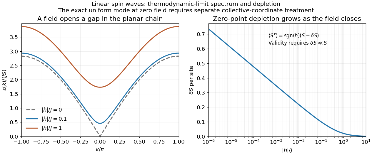


Use the unitary discrete Fourier transformThe transformed operators obey . The hopping terms contribute to the number coefficient. In the pairing sum, the odd sine part cancels between and . ThuswhereThe factor one half in the full momentum sum avoids counting an anomalous pair twice. For , for every allowed momentum. SetReal even angles ensure consistency between opposite momenta, and preserves the canonical commutation relations. The anomalous coefficient becomes . Normal ordering then giveswithThe field-polarized planar ferromagnetic spin wave has energy gap . The momenta run over the whole Brillouin zone once, including the self-inverse momenta and, for even , ; these use single-mode squeezing rather than introducing an extra independent partner.
The zero-field case has a zero-mode obstruction to bosonic Bogoliubov diagonalization. Its nonzero-momentum modes have , but , so no finite squeezing angle exists for the uniform mode. With , its Hamiltonian is , not an identically zero oscillator. For example, its matrix element between the vacuum and the two-boson number state is , whereas would vanish. Consequently the requested oscillator diagonalization is literal for nonzero field; at zero field treat the collective orientation separately or introduce a field regulator before taking a limit.
Choose the local positive axis along the classical spin. For nonzero field, a proper rotation isIt preserves the Spin commutation relations and turns the field term into . At zero field choose the classical direction , so . Expanding about the original axis without this rotation would put the reference state away from the classical minimum and would not give a controlled small-deviation expansion.
To the required order,The longitudinal exchange gives on each bond. The transverse exchange givesFinally the field contributes its classical constant and . Each site belongs to two bonds, so after removing the order- constant,These are the order- terms; the discarded products of number operators and the next square-root terms are order for occupations held fixed as . A different transverse-axis phase can reverse the sign of without changing the spectrum, but the sign above follows from the stated rotation and oscillator convention.
The Holstein–Primakoff transformation realizes a spin algebra using bosonic creation operators and bosonic annihilation operators. A boson counts a unit of spin deviation from the local positive quantization axis: with . The square root in supplies the correct spin-ladder matrix elements. In particular,Their commutator is on every physical number state, reproducing the Spin commutation relations. Although the oscillator Fock space is infinite, the physical subspace is onlyThe order of the square root and oscillator operator matters in obtaining these coefficients.
When the spin deviations are dilute, expand the square root in . The leading transverse operators are linear in the bosonic creation operators and bosonic annihilation operators and turn exchange interactions into a quadratic Hamiltonian, which can be diagonalized. Higher powers describe interactions between spin waves. The method therefore organizes corrections by inverse powers of about an ordered classical configuration. Large alone is insufficient: the average depletion must remain small compared with . Possible problems include the occupation constraint after truncation, noncollinear order requiring site-dependent axis rotations, zero modes, and infrared fluctuations that destroy the assumed dilute expansion.
There are unlisted articles, also show them or only show them.