
Varying the real scalar field gives the Euler-Lagrange field equation . Since , the answer isFor , introducing gives , the Sine-Gordon equation. The proposed real localized kink requires ; arbitrary real do not guarantee that condition. In what follows put . The displayed potential itself requires , unless a limiting prescription is specified.
For , expand the exact expression:At asymptotically short time, translational diffusion dominates if . A ballistic window occurs when , provided these scales are separated. The swimmer then retains nearly constant direction.
For and , the oscillatory exponential decays andAt intermediate times, the angular drift bends persistent trajectories into arcs. If , several rotations occur before orientational decorrelation, producing oscillatory shoulders rather than a long straight ballistic regime. In the limit , , the active contribution is bounded and periodic: . At , it remains ballistic forever, so ordinary late-time active diffusion does not follow.
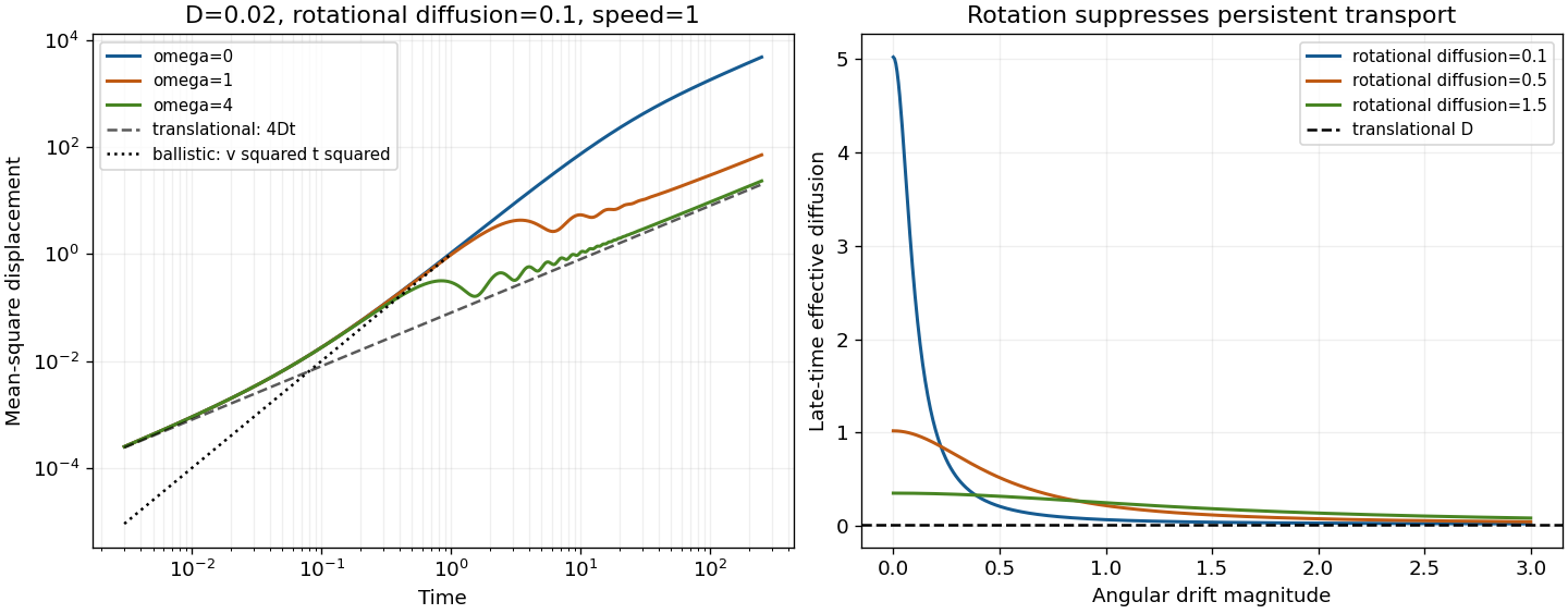

Integrate the two velocity factors over the time square . The white noise contribution is . The orientation contribution depends only on the time separation, givingThis double-integral derivation fixes the delta contribution without ambiguity about a half-weight at an endpoint. Put . Elementary integration givesUsing and multiplying out the second term yieldsThe constant and decaying terms cancel at , as required. The apparently singular case is evaluated from the integral, giving .
Use the unwrapped angle on the real line. Integrating its Langevin equation gives , where is a centered Gaussian random variable with variance . ThereforeA wrapped angular difference is bounded and would not satisfy this formula.
For the orientation correlation, . The characteristic function gives , soThe translational noise is independent of the orientation, hence the cross terms vanish. Summing its two component correlations gives . Consequently, for ,The extension to negative time uses . Because the position contains Brownian motion, the instantaneous noise velocity and its correlation are distributions; the delta contribution is not a finite ordinary velocity at .
The term is directed self-propulsion at fixed speed, while the two components of generate translational Brownian motion with diffusion coefficient . The angle has systematic angular velocity and rotational diffusion coefficient . With independent standard Brownian motions, the precise stochastic differential equations areIndependent translational and rotational noises are the usual interpretation; the supplied autocorrelations alone would not specify arbitrary cross-correlated noises.
The complete state is a Markov process: its future increments depend only on its present state and independent future noise. Its generator is . Position alone generally lacks the Markov property, since an unobserved current orientation carries memory into future displacements. At long scales orientation averaging produces the effective positional diffusion equation in solution.
Write and . With two identical degree- vertices, let lines join them. The remaining half-edges on each vertex form self-loops. Both and are even. The number of Wick contractions issince one chooses and matches the joining half-edges and then pairs the rest independently. Dividing by the expansion denominator gives every symmetry factor weight without guessing graph multiplicities.
For two quartic vertices, givesThe graphs are respectively the product of two first-order two-loop graphs; two vertices joined by two lines with one self-loop on each; and two vertices joined by four lines with no self-loops.
For two sextic vertices, givesThe corresponding numbers of self-loops on each vertex are . All seven second-order graphs are drawn in solution; in each series the graph is disconnected and the others are connected.
For completeness, a mixed quartic-sextic pair, not needed for the two pure second-order coefficients, contributesTaking removes the products of first-order graphs, that is, the terms. The requested partition function retains them.
Set the external source to zero in solution and apply Wick's theorem. At a single quartic vertex, the four position insertions have three pairings; at a single sextic vertex, six insertions have pairings. ThusThermal time-translation invariance makes this , with from solution. If desired the absolute corrections follow by multiplying by the free partition function .
The first Vacuum Feynman diagram is one quartic vertex carrying two self-loops, with weight before time integration. The second is one sextic vertex carrying three self-loops, with weight . No disconnected subtraction is appropriate for itself. The top row of the following figure shows these first-order terms and the conventions for solution.
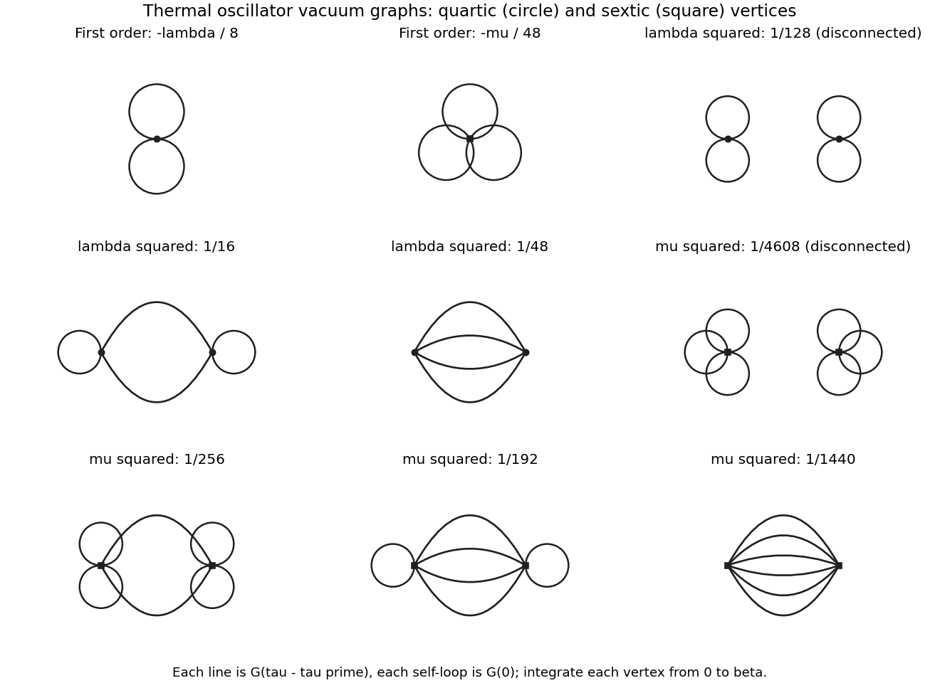
Quartic and sextic oscillator vacuum graphs through second order; the displayed coefficients include factorials and vertex interchange, and each vertex is integrated over the thermal circle
. Details. 
Keep the same measure normalization as in the free generating functional and defineHere is the source-dependent partition function, despite the common alternative convention in which that letter denotes its logarithm. A functional derivative of brings down one factor at the differentiated point. Expanding the interaction exponential and replacing each such factor by therefore givesCompleting the square in the free Gaussian integral gives because with periodic boundary conditions. Restoring replaces the upper limit by and the interaction coefficients by and , exactly as in the source.
The free Euclidean action has inverse propagator . Therefore the thermal Green's function obeyswhere is the periodic Dirac delta function. It is continuous, has continuous first derivative away from its source, and satisfies . These conditions follow by integrating the differential equation across the source and using the bosonic thermal trace.
For , solving the homogeneous equation on and imposing these conditions givesIn particular . Equivalently with bosonic Matsubara frequencies .
Here the imaginary-time Heisenberg picture position operator is , where . Bosonic time ordering places the larger imaginary time to the left without an exchange sign. The brackets denote the normalized thermal expectation valueThe trace is cyclic and is time independent, so the two-point correlation function depends only on the time difference and extends periodically with period . This periodicity is a property of the thermal correlation function, not the operator identity .
Use . Taking the trace of the imaginary-time time-evolution operator identifies the initial and final position, giving the path integralThe measure includes integration over the common endpoint. The paths are real periodic bosonic paths on the imaginary-time circle, not paths with fixed zero endpoints and not only classical trajectories. The kinetic measure is defined by time slicing; typical contributing paths need not be differentiable. For the free expansion assume . The interacting partition function requires a potential bounded below; otherwise the following formulas have the meaning of a formal perturbation series about the free harmonic oscillator.
Use the unitary discrete Fourier transform , where . Thenwith and . The factor accounts for the duplicated pair in the full momentum sum.
Make a bosonic Bogoliubov transformation . Its coefficients preserve the canonical commutation relation because . The coefficient of the pair term vanishes when . ThusThe dropped constant is in addition to the classical ground-state energy. Since , at every , so the bosonic Bogoliubov diagonalization is stable. The minimum occurs at and gives the energy gap . In the isotropic limit the pair coefficient vanishes and the familiar quadratic small- ferromagnetic dispersion relation is recovered.
Choose the positive- reference ground state and use the cyclic rotationThis is a right-handed permutation, so it preserves the spin commutation relations. It puts the ordered direction along the Holstein–Primakoff transformation's quantization axis. To the required order,The longitudinal exchange contributes . The transverse terms contributeDropping the constant and all terms of order or smaller gives the stated linear spin-wave approximation, withThe anomalous pair terms are present because the two transverse couplings differ. A different right-handed choice of transverse axes can change the sign of by a boson phase convention, while leaving the dispersion relation unchanged.
The Holstein–Primakoff transformation replaces each finite-dimensional spin algebra by a bosonic creation operator and annihilation operator, while restricting the local occupation number to . The number counts deviations from the fully polarized reference quantum state. Its zero-boson Fock vacuum has .
The representation is exact on this physical subspace: the ordered square root gives and , reproducing the spin commutation relations. For ,so the leading Hamiltonian is quadratic in bosons and describes spin waves.
The square root generates boson interactions beyond leading order and its operator ordering matters. Truncation also enlarges the Hilbert space to unphysical occupations unless the low-density approximation remains self-consistent. Large fluctuations, particularly near a gap closing or in low dimensions, can invalidate the linear spin-wave approximation even when its algebraic manipulation is straightforward.
The Hamiltonian has the discrete symmetry described in solution, whereas either selected easy-axis ground state has a nonzero order parameter and is not invariant under it. This is spontaneous symmetry breaking: the equations preserve the symmetry while the selected macroscopic quantum state does not.
An infinitesimal longitudinal magnetic field selects one orientation. The defining order of limits isin the ordered zero-temperature phase, with the opposite sign for . A symmetric finite-volume quantum state can instead have zero magnetization. Quantum ordered states are generally dressed by fluctuations rather than exact fully polarized product states, because unequal transverse exchange can create pairs of spin waves. Discrete easy-axis symmetry does not imply a gapless Goldstone mode; indeed solution finds a nonzero spin wave gap. Nor does this argument assert positive-temperature order in a one-dimensional short-range chain.[ref]
Statistical Field Theory by David Tong. Section 1.2.1, spontaneous symmetry breaking and the order of thermodynamic and zero-field limits
For a uniform classical spin with , the energy per bond isThe strict inequalities among the couplings make the direction the unique easy axis. ThusThese uniform configurations are also global classical minima: the largest singular value of the diagonal exchange matrix is , so each bond has energy at least , and both configurations saturate that bound.
A global rotation by about the axis sends to , preserves every exchange product, and exchanges the two ground states. A rotation about does the same. The broken discrete symmetry can be represented by either operation.
Let be the base-spin insertion matrix. In the eigenbasis from solution, its diagonal matrix elements vanish: . Hencenot only at large but for every finite ring at zero field.
This vanishing is not merely an averaging artifact hiding a finite-temperature ordered phase. The two-point correlation function is . In the thermodynamic limit it becomes , with finite correlation length for every and . Thermal domain walls destroy long-range alignment in this one-dimensional short-range system. At zero temperature, the two fully aligned ground states are degenerate; that limiting case must be distinguished from any fixed positive temperature.
For the sawtooth Ising chain, each apex spin occurs in only one triangle. Put . Summing that spin first gives the effective transfer matrixIn the ordered basis this isIts symmetric and antisymmetric eigenvectors are and , with eigenvaluesConsequentlyAt , the result is , correctly counting independent Ising spins. As , , the energy of three satisfied ferromagnetic bonds per two sites.
For each pair of adjacent spins, define the transfer matrix for a classical spin chain by . Multiplying its entries gives the Boltzmann factor of a whole configuration. The periodic boundary condition identifies the last index with the first, soThe assumed interchange symmetry of makes a real symmetric matrix, hence it has an orthonormal eigenbasis. At finite positive temperature, every matrix entry is strictly positive, so the Perron–Frobenius theorem supplies a unique positive largest eigenvalue , larger in modulus than every other one. Therefore .
Local observables become matrix insertions. For example, with ,Thus partition functions and correlation functions reduce to a fixed-dimensional eigenvalue problem, rather than a sum over exponentially many microstates.
Let and sum over all configurations of the Ising spins. The canonical partition function and Helmholtz free energy per site areBoth spins in each cell count as sites. In particular the denominator is , rather than .
The mean spin magnetization per site is the Boltzmann distribution averageEquivalently introduce a uniform magnetic field through and differentiate:This convention absorbs the microscopic magnetic moment into . Simultaneous reversal of every spin leaves invariant and changes the sign of the numerator, so at zero field for finite .
There are unlisted articles, also show them or only show them.