
Set the time derivatives in the master equation to zero. The first and third rows give and . Normalization then gives, with ,These expressions assume positive rates, or a limiting choice for which and the stationary distribution is unique. If rates vanish so that multiple closed classes appear, the initial condition can matter.
The word “equilibrium” in this part must mean a stationary distribution. With positive the one-way contact transitions support a nonzero stationary electric current, so the process is not in thermodynamic equilibrium and does not satisfy detailed balance. In particular, carries positive probability flow while the direct reverse rate is zero.
Write the probability column vector as , with denoting the uncharged state. The arrows in the original figure give transitions at rate , at rate , at rate , and at rate . Exclusion of double occupation means injection occurs only from state . Thus the master equation isFor example, . Every allowed jump adds to one probability and subtracts from another, which verifies the zero column sums.
Here is the probability of occupying state , and for is the transition rate from to . More precisely, over that transition has probability . This is a time-homogeneous continuous-time Markov chain: the present state contains all information needed for the next transition, the rates do not depend on time, and finite rates make multiple jumps have probability . In a physical rate description, untracked coherent dynamics or memory must be negligible on the timescale being modeled.
The master equation separates incoming and outgoing terms:Columns, rather than rows, sum to zero with this indexing. These conditions preserve normalization and nonnegative probabilities. For infinitely many states one also needs a well-defined nonexplosive process. Detailed balance is an additional equilibrium condition, not a general requirement on a master equation.
Let and . Since , the continuum minimum of the dispersion relation isFor , the energy gap closes at a positive , at wave vector . Below it, the quadratic expansion about the polarized state has a negative mode and is no longer a stable ground state approximation; higher-order terms and a different ordered reference state are needed.
Two qualifications are required by the actual assumptions. First, is permitted, in which case ; it is a concrete counterexample to the printed strict inequality . Second, a finite ring only has discrete momenta. Its finite-ring spin-wave threshold with antisymmetric exchange isThis approaches in the thermodynamic limit and equals it when is allowed. For example, and give , since the maximum of is one. Thus the continuum formula and its positive threshold require the large-ring interpretation. The two symmetry-related polarized ground states already have equal exact energy; the calculated energy gap refers to excitations about one chosen orientation.
Choose the unitary discrete Fourier transformThe finite-sum orthogonality identity gives . It also gives . Substituting from solution therefore gives the dispersion relationUsing the opposite sign in the Fourier transform reverses and the sine term together, without changing the spectrum.
For every , so the ground state of this quadratic Hamiltonian is the bosonic vacuum, for every . In the original spin variables it is the fully polarized product state. Its energy is zero after the constant subtraction. Repeating the construction about the fully polarized state describes the other easy-axis sector of the original Hamiltonian.
A one-magnon excitation has energy above the reference ground state. A normalized many-magnon Fock state with occupations has excitation energy , within the dilute regime of the linear spin-wave approximation. The lowest excitation in this sector has the minimum allowed .
Expand around the polarized ground state. With fixed as , the Holstein–Primakoff transformation gives , and . The longitudinal exchange contributesUseThe transverse exchange then gives , and the Dzyaloshinskii-Moriya interaction gives . Discarding the constant and all interactions yieldsHere periodic boundary conditions make each occur twice in the longitudinal sum. The approximation is the linear spin-wave approximation, controlled by small local magnon occupation compared with .
The Holstein–Primakoff transformation maps the finite spin basis to bosonic Fock states with . Thus is the fully polarized reference state, and creating a boson lowers by one. The physical subspace has the Holstein–Primakoff occupation constraint , not the whole infinite oscillator Hilbert space.
The specified ordering of the square root givesThese are the exact spin ladder operator matrix elements; in particular, the lowering amplitude vanishes at . The underlying oscillator obeys its usual canonical commutation relation on the enlarged space, while the spin operators preserve the constrained physical subspace. Projecting the oscillator operators themselves to a finite space would change their commutator at its upper endpoint.
Expanding converts an ordered spin problem to approximately free magnons, with interactions in higher orders of . Two complications are the nonpolynomial, order-sensitive square roots, which generate interacting bosons, and loss of the occupation bound when a truncated expansion uses the full bosonic Fock space. Large depletion, high temperature, or soft modes near a phase transition can invalidate the assumption even when is large.
The continuous internal symmetry is a common rotation around :Both the transverse exchange and the Dzyaloshinskii-Moriya interaction contain one raising and one lowering spin operator, so the phases cancel. Equivalently, and the continuous group is U(1).
The discrete internal symmetry is time reversal, , together with . Each term in contains two spin operators, so it is invariant. The operation is antiunitary; treating the reversal of all three spin components as a unitary rotation would violate the spin commutation relations. It reverses the magnetization and interchanges the two easy-axis ordered orientations. A convenient equivalent representative, composed with a rotation, is , which reverses while preserving as operators.
The statement about one continuous and one discrete internal symmetry describes generic parameters. At , additional unitary rotations about transverse axes are allowed; at , the continuous internal symmetry enlarges to full spin rotation symmetry. Spatial translations of the uniform chain are separate symmetries of the sites.
For one triangle, equal base spins give energy . Their minimum occurs at and is . Opposite base spins give energy , independently of the apex spin. The all-equal configurations have energy .
When , the six configurations with precisely one spin different from the other two all have minimum energy . For a fixed first base spin, there is one minimum choice if the next base spin is the same, and two choices of apex if it is opposite. The ground-configuration counting transfer matrix is thereforeThis ground-state counting of the frustrated sawtooth Ising chain proves the extensive geometric frustration and the residual entropy .
When , . Every triangle must have equal base spins and the opposite apex spin. Shared base spins propagate that choice around the chain, leaving just two global ground states, of energy . Their entropy per spin is .
For couplings favoring ferromagnetism, write , with . Both orientations of an all-equal triangle minimize every bond simultaneously. The common base spins then make the whole chain uniform. There are two global ground states for either or , so no corresponding distinction in residual entropy occurs. This statement assumes all bonds remain nonzero.
Differentiate the Helmholtz free energy at fixed couplings. With from solution, the entropy per spin isIt is particularly useful to writeAt , this is , so . For fixed , the first exponential dominates alone, giving . Hence the residual entropy isThe finite positive difference must be kept fixed in the second limit; taking it to zero first gives the other answer.
At high temperature, and , whenceAll configurations become equally probable because their Boltzmann factors tend to one. The two available states per spin, rather than the coupling values, determine this entropy.
In the basis the transfer matrix and its eigenvalues areFor finite positive temperature, and . Consequently and in the thermodynamic limit. There are spins, so the Helmholtz free energy per spin isThe factor is essential: one transfer matrix step counts two spins. For completeness, if the undefined is retained, set , and . The same thermodynamic limit gives whenever these are two distinct spin values.
For the sawtooth Ising chain, there is a source inconsistency: the printed Ising spin values are , with no definition of . The requested transfer matrix follows for , namely the usual Ising model with values . For arbitrary , summing an apex spin actually givesFor example, , and give the bracket , whereas the claimed hyperbolic cosine gives . Thus the printed identity is false literally. The rest of Question 1 uses the intended symmetric Ising spin values, .
For a fixed configuration of base spins, each apex spin appears in only one local Boltzmann factor. The apex spins are therefore conditionally independent, and their finite sums factorize:Only the base spins carry information from one triangle to the next. The apex spins have already been summed out, so no apex index remains in the transfer matrix; the final trace implements the periodic boundary condition.
Take and hold fixed. The heat capacity comes from the minimized free energy, , with any smooth background added separately. For and ,Above , and the polynomial contributes zero. There is a finite jump, rather than a divergence: the conventional ordinary mean-field critical exponents areThe upper branch has zero order-parameter contribution; a finite regular heat capacity has exponent zero.
Along the tuned tricritical path , the ordered minimum givesUpper-side qualification: the vanishing disordered-side heat-capacity amplitude in Landau theory matters here: for and , the minimizing solution is still exactly , so this saddle-point polynomial gives and . A zero function cannot determine a nonzero-amplitude power-law exponent. For example, adding the allowed smooth background , with , leaves the entire phase diagram unchanged but makes the upper-side heat capacity exactly , not a divergence.
One convention assigns the tricritical scaling exponent to both sides, writing with at this mean-field approximation saddle. If the source's literal is meant to have a nonzero leading coefficient, the given polynomial establishes no upper-side tricritical singular exponent; with a nonzero smooth background its leading upper-side exponent is zero. A nonzero upper-side singularity requires fluctuation information beyond this minimization. This distinction prevents claiming an upper-side divergence that the displayed Landau free energy does not produce.
Write , , at fixed , and define the critical exponent by on the ordered side. For fixed and small negative , the stationary equation gives . ConsequentlyAt the tricritical point approached along the tuned path , the stationary equation instead gives , soFor fixed , the transition occurs before reaches zero and the magnetization jumps; it is not a second-order transition and has no vanishing-order-parameter exponent of this form. A path that does not keep the quartic coefficient tuned to zero generally crosses over to the ordinary result.
Fix . Stationary points satisfy . With , the nonzero candidates areKeep only real positive roots. At such a point,so gives local minima and gives local maxima when both exist. The solution is a local minimum for . To choose the phase, compare free energies: using the stationary point relation givesFor , this expression is negative whenever a nonzero stationary minimum exists. The paramagnetism phase is stable for , and the ferromagnetism phase with is stable for . The phase transition at , , is continuous and second order.
For , equality with requires . Substitution into the stationary equation gives the first-order coexistence curveThe disordered phase is the global minimum above this curve, and the ordered phase is the global minimum below it. At coexistence the factorizationexhibits three equally low minima, and , proving the discontinuous jump.
The ordered spinodal is , , where its local minimum meets the intervening local maximum. The disordered spinodal is , . Thus the ordered phase is metastable for ; the disordered phase is metastable for . These spinodals are limits of metastability, not equilibrium transition curves.
The first-order curve meets the continuous transition line at the tricritical point . On the specially tuned path , the equilibrium ordered solution is for and tends continuously to zero at the origin.
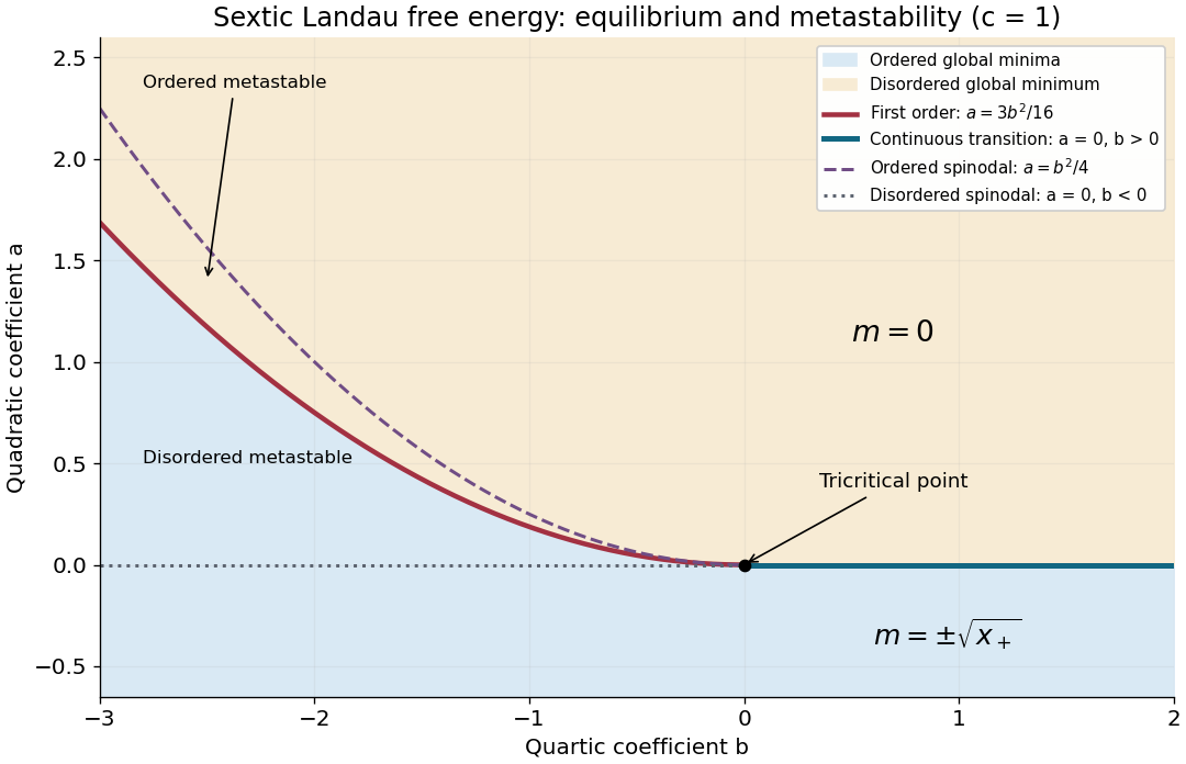
Phase diagram of the sextic Landau free energy, including coexistence, spinodals and the tricritical point
. Details. 
For the sextic polynomial to be bounded below at large while allowing either sign of , its leading coefficient must obeyIf , the free energy tends to as , so it cannot define an equilibrium within this truncation. The exceptional case is stable for and gives the ordinary quartic Landau theory; it cannot stabilize the negative- region required for the full sextic phase diagram. Higher positive powers could stabilize a negative , but they are absent from this model.
Choose a coarse-grained magnetization as the order parameter: it vanishes in the paramagnetism phase and develops a spontaneous nonzero value in the ferromagnetism phase. In zero applied magnetic field, spin reversal sends , so the local Landau free energy contains only even powers. A minimal spatially inhomogeneous free-energy functional isThe positive gradient coefficient penalizes rapid spatial variations. Near an ordinary transition take , , and positive ; retain the sextic term when can approach or cross zero. The source is conjugate to the magnetization and explicitly breaks spin reversal.
Determine equilibrium by minimizing this free-energy functional, imposing the appropriate boundary conditions. Its Euler-Lagrange equation isFor a uniform system at , compare the values of all stable stationary solutions, rather than accepting every solution of this equation. The selected global minimum gives the equilibrium magnetization; derivatives of its free energy give entropy, heat capacity and magnetic susceptibility. At an ordinary transition the two ordered minima emerge continuously from zero. Spatial dependence also permits domain walls and an estimate of the correlation length.
This is a mean-field approximation: it selects a minimizing profile and neglects statistical fluctuations around it. The symmetry constrains the expansion, but its numerical coefficients are phenomenological. Close enough to a transition, thermal fluctuations near a critical point can invalidate the resulting mean-field critical exponents.[ref]
Statistical Field Theory by David Tong. Chapter 1, the Landau-Ginzburg free-energy functional, spatial gradients and mean-field phase transitions
Since every quasiparticle energy is positive, the ground state is the vacuum of all the annihilation operators, including . Its zero-momentum mode is therefore empty. For each positive momentum, the inverse Bogoliubov transformation givesBoth annihilate the normalized pair state . For example, applying produces the two cancelling terms . ThusThe factors have even fermion parity and commute for disjoint momentum pairs. Each normalized factor is a superposition of zero and two fermions, whose pair-occupation probability is . ThereforeThere is no zero-mode contribution. For fixed , the sum converges since .
A normalized simple excited state is for . Its excitation energy is , and its total momentum is : both terms in add momentum . Acting on the pair givesThe affected pair now contains exactly one fermion instead of mean number ; all other pairs are unchanged. ConsequentlyThis is the fermion number of a Bogoliubov excitation. Its change in mean fermion number lies between zero and one for , with the value one at . The Bogoliubov quasiparticle coherently mixes adding a fermion and removing the opposite-momentum fermion; it is not an eigen-excitation of the original fermion number operator. Indeed,so fermion number is not conserved when , while fermion parity is conserved. The generally noninteger change is an expectation value in a coherent paired background, rather than a fractional eigenvalue of the fermion number operator. In the weak-pairing limit at fixed , it tends to one, as expected for an ordinary added fermion.
Group the nonzero modes into independent pairs . For one pair set , and introduce the Nambu spinor . Normal ordering using givesThis exactly contains both kinetic terms and the pairing terms once; there is no additional factor of one half because only is summed.
Insert , where and is the Bogoliubov transformation matrix. Direct matrix multiplication yieldsChoose the diagonalizing branchThen the off-diagonal terms vanish and the upper diagonal entry is . Extend the angle to negative momenta as in part b; the sine relation just written applies to the positive representative of each pair. The BCS coherence factors can be chosen asHere denotes , and denotes ; these expressions are nonsingular because and . The minus sign of for positive is fixed by the pairing phase in this Hamiltonian.
A second use of the canonical anticommutation relations givesThe zero-momentum term was never paired and is simply . HencewithThe constant is the ground-state energy. At fixed , its ultraviolet tail converges: in one dimension. Replacing by would incorrectly pair a spinless mode with itself.
For real angles write and . For one independent pair , the transformation and its conjugate readUsing the canonical anticommutation relations for the modes givesThe remaining anticommutators vanish for independent momentum pairs. The displayed two-by-two matrix is unitary and its inverse is obtained by changing to .
When the same formula is indexed over both signs of momentum, its first row at must agree with the conjugate of its second row at . Thus a consistent global convention requiresThis is the odd-momentum fermionic Bogoliubov angle convention. If one checks only the first-row formulas, their cross anticommutator is ; its vanishing gives the condition modulo , with possible signs absorbable in the modes. Requiring both rows to describe the same operators fixes the convention above. Merely checking a separate unitary matrix at each momentum misses this redundancy: choosing in both first rows would give .
At , the annihilation operator and its conjugate belong to one mode. The full displayed formula is consistent only with ; choose and . This mode is not a two-mode pair.
There are unlisted articles, also show them or only show them.