
In units , a free homogeneous scalar has and therefore a stiff equation of state. Its equation gives , while the Friedmann equation gives . The displayed contracting branch satisfies both equations for negative conformal time. Constant normalizations and an additive scalar shift can be restored.
The conservative equation has a saddle loop with for . Its homoclinic orbit integrals are and . Substitution evaluates them as displayed. For a weak perturbation , integrating the energy derivative gives , hence . The nonzero derivative makes this a simple first-order splitting zero.
If the spectrum of an element lies in the open right half-plane, holomorphic functional calculus gives the displayed square root with spectrum in that half-plane. It is unique there. Two such roots have character values equal to the unique scalar square root with positive real part. Every character of an algebra is therefore nonzero on , so the character description of the spectrum makes invertible. From one obtains . Equal character values alone do not prove equality in a possibly nonsemisimple algebra.
If the spectrum of an element avoids , its holomorphic functional calculus value for the principal cube root is the unique with and spectrum in . For uniqueness, any other such defines a continuous unital algebra homomorphism from the slit-plane holomorphic functions to the algebra. It sends the coordinate to , so continuity and uniqueness of holomorphic functional calculus identify it with . Applying it to the principal cube root gives . This argument does not assume commutativity of the ambient algebra or separation by algebra characters.
Banach algebra exponential 2026-10-14
The exponential series converges absolutely in a unital Banach algebra. Multiplication of absolutely convergent series gives , and gives when commute. Termwise differentiation gives near zero. In a C-star algebra, if and is real, taking adjoints termwise gives , so this exponential is a Unitary element of a C-star algebra and has norm one. These facts let a norm bound on a functional recover its real values on Hermitian elements.
If a spectrum of an element splits into disjoint nonempty compact pieces , choose disjoint open neighborhoods and a holomorphic function equal to one on the first and zero on the second. The holomorphic functional calculus sends it to an idempotent with the corresponding zero/one values under every algebra character. It is neither zero nor identity: if one piece were killed, a reciprocal function on the other piece would make an originally spectral coordinate difference invertible.
If a compact spectrum of an element avoids zero and zero belongs to its unbounded complementary component, choose a simple arc from zero to infinity avoiding the Banach algebra spectrum. Its complement is a simply connected neighborhood of the Banach algebra spectrum, admitting a holomorphic logarithm. Apply holomorphic functional calculus to that logarithm and the composition rule for holomorphic functional calculus to the exponential to obtain the displayed identity. An invertible matrix over the complex numbers always satisfies the hypothesis because its finite Banach algebra spectrum cannot separate zero from infinity.
Hölder exponent 2026-10-14
The Hölder exponent in Hölder continuity measures the power in the bound . For , a larger exponent imposes stronger local regularity on bounded distance ranges. Exponent one is Lipschitz continuity.
Hoeffding confidence interval 2026-10-14
For a fixed positive sample size of independent and identically distributed Bernoulli random variables, letThe Hoeffding inequality makes a conservative confidence interval for : for every . Indeed, exclusion from the closed interval implies , an event contained in the deviation event bounded by . Clipping to retains coverage because already lies there. For , , and an observed frequency , , giving approximately .
Coverage concerns repeated independent samples: the unknown is fixed and the confidence interval is random. This fixed- guarantee does not justify repeatedly checking the same bound and stopping as soon as it looks favorable. The Hoeffding sample size for Bernoulli frequencies chooses in advance; guarantees across repeated inspection times require separate control of the additional events, for example through a union bound with an allocated failure probability at each time.
Hoeffding sample size for Bernoulli frequencies Created 2026-10-14 Updated 2026-10-31
Let be independent and identically distributed Bernoulli random variables with success probability , and let be their observed frequency, a sample mean. Since every interval width is one, . Substituting into the Hoeffding inequality givesFor tolerance and failure probability , solving yields the sufficient sample sizeHere is the natural logarithm. For and , guarantees an error smaller than with probability at least , for every . The two-sided bound at this sample size is approximately . A specified single direction instead needs , or for these choices. Halving the tolerance multiplies the unrounded sufficient sample size by four; reducing the failure probability tenfold adds before rounding.
This is a conservative sufficient sample size, not a necessary minimum. For a specified , the count has a binomial distribution, whose exact upper tail probability isFor , the Hoeffding inequality bounds this by . An arbitrary frequency threshold uses ; if , the event is impossible. The discreteness of the count and its variance can make the exact tail probability substantially smaller. At , , , the exact upper tail probability is about , while the bound is . At , , the same deviation gives the same bound but an exact upper tail probability about .
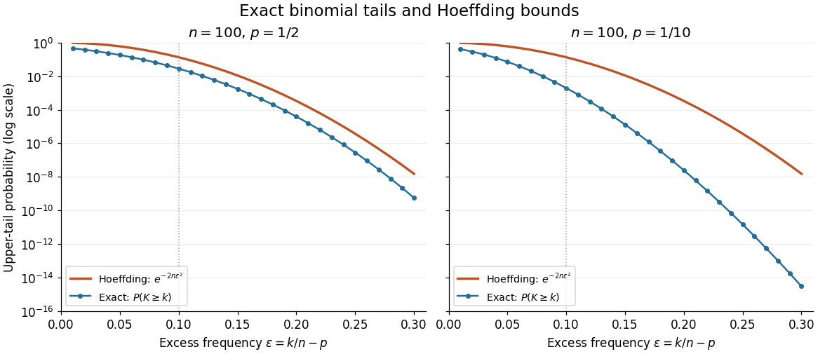
Exact binomial distribution tails compared with the Hoeffding inequality
. Two original specified models, each with independent Bernoulli trials. Each dot includes its integer threshold , with horizontal coordinate . Exact finite sums are evaluated with rational arithmetic before conversion for plotting. The Hoeffding inequality uses the width one in both panels; it does not use the smaller variance at . These are model probabilities, not measured frequencies. Details.
Let a surjective morphism from a smooth projective surface to a projective surface contract an irreducible curve . Pull back an ample divisor from the target to obtain . The projection formula for algebraic cycles gives and . The Hodge index theorem for algebraic surfaces makes the intersection form negative definite on the orthogonal complement of this positive-square class. Since an ample divisor on the source meets positively, its numerical class is nonzero, and .
Second Hochschild cohomology classifies split square-zero extensions Created 2026-10-14 Updated 2026-11-05
Fix an -bimodule . A unital ground-ring-linear split extension with square-zero kernel can be identified with , with multiplication . Associativity is exactly . Changing a unital linear section by changes by . Thus equivalence classes of these split extensions are . Over a field every such vector-space extension splits; over a general ground ring a splitting hypothesis is essential for this ordinary cochain classification.
Over a field, the bimodule resolution is exact: multiplication identifies the quotient by , and that element is a non-zero-divisor in the two-variable polynomial ring. Applying the bimodule Hom functor gives zero differential, proving the displayed Hochschild cohomology. Degree-one classes are the derivations .
The ordinary Hochschild cochain complex is defined using a chosen commutative ground ring . The bar complex is exact via insertion of , but its terms are projective over the enveloping algebra when is projective over , in particular when is a field. Without that hypothesis the ordinary cochain groups compute relative Hochschild cohomology and cannot automatically be identified with absolute Ext. Likewise, ordinary second cohomology classifies ground-ring-linearly split square-zero extensions, not arbitrary nonsplit ring extensions.
// Destination: module-theory.bigb
Maximum occupation is not a hitting probability Created 2026-10-14 Updated 2026-11-05
For with and standard Brownian motion, the one-time occupation Probability is . It is maximized at , giving . The actual hitting probability is . To derive it, solve on with , , obtaining , and let . A path that reached the level and returned contributes to the latter event but not to a given one-time tail.
Two Hilbert space modules are unitarily equivalent if each embeds isometrically as a closed submodule of the other. For isometric intertwiners and , let and . These summands are orthogonal. The operator acting as on and as on is the required unitary onto .
The gauge-covariant kinetic term of the Higgs doublet gives . Differentiation with respect to the external fields yields Feynman rules for one Higgs boson and two matching massive electroweak gauge bosons, and for two Higgs bosons and the same pair. Identical neutral fields supply combinatorial factors. The neutral radial Higgs boson has no corresponding elementary coupling to photons at tree level.
Goldstone-boson equivalence theorem Created 2026-10-14 Updated 2026-11-05
At tree level and energies much greater than a gauge-vector mass, an amplitude with longitudinal external gauge bosons equals the corresponding amplitude with their would-be Goldstone bosons, up to conventional external-state phases and relative corrections for a nonzero leading amplitude. In a renormalizable gauge, the broken-symmetry identities relate to ; inserting explains the result. Loop-level versions include field-normalization factors. This is different from an equivalence theorem for field redefinitions.
Shifted quartic Higgs potential normalization Created 2026-10-14 Updated 2026-11-05
In unitary gauge, , so this Higgs potential gives , a cubic coefficient and a quartic coefficient . The corresponding Feynman rules are and . Writing the potential with an additional factor changes the relation between its named coupling and the Higgs boson mass; it does not change these mass-based rules.
Higgs radial mass for a half-normalized quartic potential Created 2026-10-14 Updated 2026-11-05
For and the canonically normalized radial field, the expansion is . Comparing the quadratic term with gives the displayed mass. Replacing the prefactor by changes the answer to , so the potential's normalization must be retained.
There are unlisted articles, also show them or only show them.