
Past exam of the mathematics course of the University of Cambridge 2001 iii Paper 28 1 Solution Created 2026-10-03 Updated 2026-10-14
For a group with sample size , let be its overweight count. The natural sampling model is a binomial distribution, , with observed proportion . A grouped-binomial logistic regression specifiesFitting event/nonevent counts, or fitting the proportions with weights , gives the same binomial likelihood. The weights represent trial counts; unweighted regression of the proportions would give small and large groups the same influence. If printed percentages are rounded, exact original event counts are preferable to manufacturing fractional counts from .
Year should ordinarily be a factor with three levels unless a linear trend over time is specifically intended. Country, sex and age group are also possible factors. The actual subset, reference levels and formula are absent from this PDF. For a year-by-age interaction term, writeWith treatment contrasts, is the baseline logit, and are effects at the reference level of the interacting factor, and is an additional difference of log-odds differences. Exponentiating a main-effect contrast gives an odds ratio; exponentiating an interaction contrast gives a ratio of odds ratios. It is incorrect to interpret a main effect as a constant effect across the other factor when the interaction term is present.
A coefficient table should be read as estimate, standard error, a Wald estimate/error ratio and its reference-distribution probability. A whole multi-level interaction term is better tested by a nested likelihood-ratio test, using the decrease in deviance and the number of added independent coefficients. Null and residual deviances, residual degrees of freedom, convergence and fitted probabilities should all be checked. Large residual dispersion suggests lack of fit or dependence within sampled schools; a quasibinomial regression or an appropriate clustered analysis may then be preferable. Residual deviance is not automatically a valid chi-squared goodness-of-fit statistic for sparse groups or after estimating a free dispersion.
An interaction plot should display the group means or fitted probabilities against year, with separate lines for the interacting factor, and should also inspect the link scale. Nonparallel probability curves alone do not establish a logit interaction: even an additive logit model transforms nonlinearly to probabilities. As an independent descriptive illustration, the original study's Table 2 reports English boys' age-specific percentages. The following original plot shows their widening age differences after 1984 on both scales. It uses published descriptive values, not a reconstruction of the absent examination fit. The data are from pmc.ncbi.nlm.nih.gov/articles/PMC26603/ .
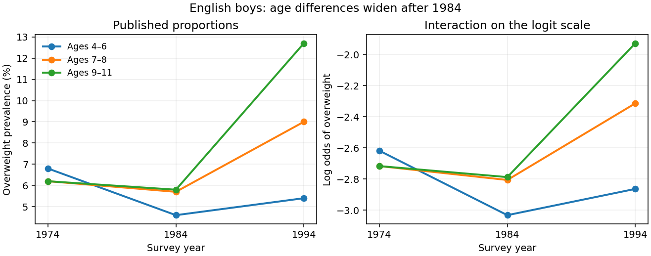
Published English boys' overweight prevalence by age and year, shown on probability and logit scales
. Details. 
For example, on the probability scale the 1984–1994 increase for the oldest group exceeds that for the youngest by percentage points using the rounded table values. On the logit scale the corresponding difference of differences isThis describes the interaction pattern, but its sampling uncertainty requires the group counts. The absent output prevents identifying the exam fit's coefficient estimates and significance tests.
There are two different uses of Poisson regression. A rare-event approximation models withThe fixed offset accounts for exposure, and exponentiated slopes are risk ratios, not odds ratios. The approximation is most appropriate when probabilities are small; it is not exact for appreciable prevalence because binomial variance is rather than .
An exact alternative stacks event and nonevent counts in each group and fits a log-linear model with a separate group intercept and event-by-predictor effects:Conditioning on their total gives the binomial event probability , whose logit is exactly . Profiling the group intercepts enforces the observed totals and reproduces the grouped-binomial logistic regression. This Poisson surrogate for a conditional multinomial model is exact and should not be confused with the rare-event approximation.
Past exam of the mathematics course of the University of Cambridge 2001 iii Paper 27 4 Solution Created 2026-10-03 Updated 2026-10-14
Record the discount level at the start of each policy year as the state. A no claims discount system is a Discrete-time Markov chain when, conditional on this state, the next year's claim behavior and update rule do not depend on earlier history. Independent annual accident and loss mechanisms with a fixed state-based reporting rule give this property; one should not equate the probability of an accident with the probability of a submitted claim.
The density identifies as a standard normal random variable: substitute and . Therefore, for ,Here is the numerical repair cost. The character preceding in the PDF is a currency symbol, not a separate multiplier.
Order states as . With the stipulated common annual probability of no submitted claims, the transition matrix isA claim resets any state to zero, while a no-claim year raises the discount one level or keeps the top level fixed. If claim probabilities depend on the state, the corresponding row instead uses ; the same transition mechanism applies. The supplied single is a simplifying model assumption.
For a policyholder currently at zero discount, the current premium has the same value under either decision and cancels in the comparison. If the repair is self-funded and no later accidents occur, the next two premiums are and , giving a total cost including the current premium. If a claim is made, the next two premiums are and , giving total cost , with the repair paid by the insurer. Thus the two-year no-claims threshold with reset to zero isAt equality the holder is indifferent; it has probability zero under the continuous density. This assumes full reimbursement and no excess or deductible, as in the stated model.
Put . The conditional expected claim is . Completing the square in the normal integral gives the truncated lognormal momentDividing by the reporting probability gives the expected size of a submitted claim for the full-premium holder:All monetary amounts must use the same unit despite the PDF's mixed currency notation. The other two current levels both have next-two-year no-claim premiums , versus after a claim, so their thresholds are . Consequently incorporating this behavioral decision into claim probabilities generally produces state-specific , rather than deriving a common from the severity density alone; no accident-frequency law is provided.
Past exam of the mathematics course of the University of Cambridge 2001 iii Paper 27 2 Solution Created 2026-10-03 Updated 2026-10-14
Write the surplus process in the classical risk model as , with positive independent claims. Condition on the first claim time, which has exponential distribution of rate . If that claim occurs at , the available capital is and survival requires its size not to exceed that capital. The independent future process then givesPut and change variables . We obtainThe convolution of bounded with the integrable density is continuous; differentiation of this expression is therefore justified. It proves the survival version of the ruin integro-differential equation:
The density is a hyperexponential distribution with mixture weights and exponential rates . Its total integral is one and its mean isThe relative safety loading means . Substitution of gives and .
Set . Differentiating in its equivalent form gives . The survival equation becomesApply the constant-coefficient operator , where . Since and ,Expanding and cancelling yields . Thus .
Positive loading also fixes the limiting boundary value . Indeed the aggregate-claims process minus premium income tends to minus infinity almost surely by the strong law of large numbers. Its supremum over all time is consequently finite almost surely, since paths have finitely many jumps on bounded intervals. The probability that this supremum exceeds tends to zero. Hence . At zero, the given value is , and the integral equation supplies the extra condition . Thereforeso and . The nonruin probability isThis is the two-exponential-mixture survival probability. It increases from to and satisfies the original integral equation, not just the differentiated equation; the zero-capital derivative condition prevents introducing extraneous solutions.
Past exam of the mathematics course of the University of Cambridge 2001 iii Paper 27 1 Solution Created 2026-10-03 Updated 2026-10-14
Where the moment-generating function is finite in a neighborhood of zero, define the cumulant-generating function and the th cumulant by . Differentiation givessince . Thus the first two cumulants are the mean and variance.
Conditional on , independence gives . Summing over the Poisson distribution yieldsHence the compound Poisson cumulants giveFor the moment statements, finite second moments suffice even when a moment-generating function does not exist near zero: conditioning gives . This distinguishes the raw second moment from the variance of an individual claim.
For a single flood, the law of total expectation and law of total variance similarly giveCondition on the number of floods and apply the same laws once more. All floods have these moments and are independent of , so the annual total satisfiesThe additional term is the variation in the number of entire flood clusters; it would be lost by treating individual claims as an ordinary Poisson stream.
For the annual count , its probability generating function isThis is the nested Poisson flood count. Differentiating, or conditioning on , gives and . Thus is not Poisson when , since its variance exceeds its mean. If either parameter is zero it is identically zero, a degenerate Poisson distribution.
Let be the number of valid claims in flood . Independent validity marking gives . Its generating function isso Poisson thinning gives . With validity independent also of claim amount, each claim contributes expected paid amount . Therefore the annual expected payment is . The independent-mark assumption is needed for this multiplication; a size-dependent invalidity rule would require the joint expected value of amount and validity instead.
Past exam of the mathematics course of the University of Cambridge 2001 iii Paper 26 4 Solution Created 2026-10-03 Updated 2026-10-14
Write for work arriving in slot and for the service rate of a queue. For a work-conserving single-server queue, the Lindley recursion is . For stable independent and identically distributed random variables with mean , its stationary workload supremum has the formDifferent scaling limits of a queue concern different quantities growing large; they need not share either a probability speed or a likely path to overflow.
For large-buffer queue scaling, fix the input law and and let the buffer size of a queue . Assume finite exponential moments around a positive root of . An overflow accumulated in slots requires an average input about , so Cramér's theorem assigns logarithmic cost . Optimizing the duration gives the Cramér-Lundberg workload exponentFor an interior root with , Fenchel–Young inequality verifies the minimization: the lower bound is because , and equality occurs at . The exponential workload bound from cumulative arrival moments gives the upper exponent for every ; an exponentially tilted positive-drift path or the duration calculation gives the matching lower exponent. In effective bandwidth notation, . This regime measures long accumulation into a large buffer with a fixed positive stability margin.
For many-source queue scaling, superpose independent copies of an input process, give the server capacity , and give it buffer size . For each lookback horizon , the average of the source cumulative arrivals has a large deviation principle with rate function . Overflow at that horizon costs . Optimizing the lookback horizon suggestsFor independent slots, , giving . The integer horizon is important in a slotted system. For temporally dependent sources, use the cumulative-input cumulant-generating function, rather than multiplying a one-slot formula by . The heuristic needs uniform control of the tail of the stationary supremum to justify optimizing an unbounded set of horizons; stability and suitable exponential-moment estimates provide this in the usual models. The growing quantity here is the number of independent sources, while per-source capacity and buffer remain fixed.
For moderate-deviation queue scaling, consider a bufferless queue with aggregate Poisson input of mean and capacity , . The spare capacity is much larger than the ordinary central limit theorem scale but much smaller than . The Poisson sample-mean rate function near its minimum has expansionWith , the cost is asymptotic to . Hence Poisson moderate deviations give . The quadratic cost comes from a shrinking neighborhood of the mean, rather than from a fixed macroscopic overload. The regime is useful for a large aggregate whose service margin lies between its typical fluctuation scale and its mean scale.
For a heavy-traffic limit of a queue, instead hold the input law fixed with mean and positive finite variance , and let with and . In slots the net input has mean about and random fluctuation of size . Thus the functional central limit theorem, followed by the Skorokhod reflection map on the half-line, suggestswhere is reflected Brownian motion with negative drift and variance parameter . The stationary law of negatively drifted reflected Brownian motion has tail . When passing the stationary distribution through the limit is justified, this predictsFor dependent input satisfying a suitable invariance principle, replace by its long-run variance of a stationary process. This regime is appropriate near critical load and on long time scales; a functional transient limit alone does not automatically justify the stationary-limit interchange.
A different large-service regime holds the input law fixed. With Poisson distribution of mean and bufferless capacity , let . The single-point lower bound and the optimized Chernoff bound for , using Stirling's formula, give the Poisson large-service overflow asymptoticHere the service rate grows while the input mean does not. A quadratic moderate-deviation approximation would describe the wrong part of the Poisson tail.
To choose a regime, compare the spare capacity, typical fluctuations, number of sources and buffer size before selecting a formula. Use the large-buffer exponent for a fixed stable input and a long overload episode; use the many-source variational cost when independent flows and resources grow together; use moderate deviations for an intermediate safety margin; use the heavy-traffic diffusion when the stability margin tends to zero; and use the fixed-input Poisson tail when service alone becomes very large. Check temporal dependence and exponential-moment assumptions. For heavy-tailed subexponential distributions, a single exceptionally large arrival can dominate overflow, so a finite exponential workload root and a Brownian approximation to the far tail need not apply. These comparisons explain why the same nominal queueing theory system can have different useful asymptotic descriptions.
Past exam of the mathematics course of the University of Cambridge 2001 iii Paper 25 4 Solution Created 2026-10-03 Updated 2026-10-14
On an -dimensional register, the quantum Fourier transform with positive-exponent convention isIt is the unitary version of the discrete Fourier transform on amplitudes. The inner product of columns is , equal to one when and zero otherwise by a finite geometric series, so the transformation is unitary.
For the qubit implementation take , write in most-significant-bit-first order, and put . Expanding separates the Fourier phase as a product. The resulting dyadic quantum Fourier transform circuit identity isIndeed the phase on output bit is , depending on the last input bits; multiplying the factors recovers and the normalization .
Implement the product in reverse wire order as follows. Process input wire , starting at . A Hadamard gate maps to . For each still-unprocessed wire , apply a controlled phase gate with control , target , and target phaseOn a computational-basis input this multiplies the target's one-component by , so the processed wire becomes exactly . Continue through all wires and reverse their order using SWAP gates. This equals the boxed transform on every basis vector and therefore on arbitrary superpositions by linearity; it does not require learning the input bits by measurement.
There are . A swap is three controlled-NOT gates, since the alternating control directions send successively to , then , and finally . Thus the exact transform uses one- and two-qubit gates from this phase-gate family, polynomial in the register size . This is a circuit-complexity statement, not a claim that all transformed amplitudes can be read out efficiently. If a fixed finite gate alphabet is required, the phase rotations must instead be synthesized to the desired accuracy; the exact count treats them as the available simple rotation gates.
There are unlisted articles, also show them or only show them.