
A scalar linear differential equation of order has the formHere the coefficients and the forcing term are prescribed functions of the independent variable . A classical solution of a differential equation is an -times differentiable function satisfying the identity at every point of its interval. The unknown function and its derivatives enter to the first power, without products between them or coefficients depending on . Equivalently, the differential operator is a linear map: for constant scalars ,The forcing term may be zero, giving a homogeneous linear differential equation, or nonzero, giving an inhomogeneous linear differential equation. Linearity of does not mean that every function graph of a solution of a differential equation is a straight line.
To use the usual order- initial value problem theory on an interval , assume that throughout and that all and are continuous functions there. Dividing by normalizes the highest derivative; specifying at then selects one solution of a differential equation throughout . A zero of needs separate analysis: one cannot divide through it and retain these conclusions. The first-order normalization appears in OpenStax's definition and standard form of linear equations; the corresponding system theorem is in MIT's existence and uniqueness notes for linear systems.
The coefficients need not be linear functions of . For example, is a linear differential equation on , although is quadratic. Its solution of a differential equation with initial condition is : its derivative is , so substitution gives , and . The zero of the highest coefficient at explains the domain restriction. In contrast, , and are nonlinear ordinary differential equations because of their dependence on the unknown function. Variable coefficients and nonlinear ordinary differential equations are different issues; see MIT's definitions and examples of first-order linear equations.
The practical benefit of linearity is that it separates the effect of the initial condition from the effect of the forcing term. Once one particular solution satisfies , every solution of a differential equation isHere is the kernel of a linear map, consisting of solutions of a differential equation to the associated homogeneous linear differential equation. Indeed, , and conversely . Thus the family for a fixed forcing term is an affine space obtained by translating . If is not identically zero, the zero function is absent, so this family is not a vector space under the usual operations on functions. This short argument explains why a general solution is a particular solution plus a homogeneous solution.
A solution of a differential equation has finite-time blowup in norm when as approaches a finite endpoint of its maximal interval of existence. This is stronger than merely approaching an excluded boundary of an open state domain while staying bounded. The finite-dimensional continuation criterion distinguishes these obstructions; for a locally Lipschitz continuous ordinary differential equation on , a finite maximal endpoint inside necessarily entails finite-time blowup.
A simple example with a smooth right-hand side isThe derivative identity verifies the equation and the initial condition. Also for , giving local Lipschitz continuity and therefore uniqueness. Yet the positive blowup time is . Computed values show the accelerating growth:The right panel under the Picard-Lindelöf theorem deliberately clips its vertical axis at : the trajectory has already left the picture at , before reaching . A plot ceiling is a display limit, not a finite value at blowup.
The tangent function also quantifies the last part of the trajectory. With ,Thus the height is approximately the reciprocal of the remaining time. At remaining times , the heights are approximately . These follow from the sine and cosine limits at zero and explain the steep rise without relying on the appearance of a clipped function graph.
The distinction is useful when interpreting a solution of a differential equation: uniqueness certifies a trajectory while it exists, while growth estimates decide how far it can be followed. For , the Lipschitz constant on a bounded state interval grows with , and the right-hand side grows quadratically. There is no global Lipschitz constant or linear-growth bound of the kind used by the finite-dimensional continuation criterion. Smoothness at every finite state is entirely compatible with finite-time blowup.
Let be an open set and a continuous function. Suppose is locally Lipschitz in the state , with a Lipschitz constant uniform on a sufficiently small time-state neighborhood of each point. Then each determines a unique local solution of a differential equation to the displayed initial value problem, on an interval around . This is the local theorem in Ordinary Differential Equations and Dynamical Systems by Gerald Teschl.
For example, , , has the solution of a differential equation : its derivative is itself and its starting value is . The Lipschitz constant is , since . Thus uniqueness follows even before computing . Picard iteration below constructs this exponential function one polynomial at a time.
The Lipschitz condition has real content. For the continuous function involving a square root,each waiting time gives a different forward solution of a differential equation:The constant solution of a differential equation is another choice. At , delays give respectively. Before the join, both sides of the ordinary differential equation are zero; afterwards, . Both one-sided derivatives at are zero, so the join is valid. All these trajectories can also be extended by zero to . The failed Lipschitz condition is visible in the quotientFor this quotient is . Continuity still allows local existence by the Peano existence theorem; it cannot choose a waiting time. MIT's 18.034 Lecture 2, Example 2.3 develops the same waiting-time mechanism for a different ordinary differential equation, .
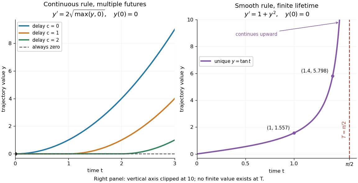
Failure of uniqueness and finite-time blowup are different obstructions
. Left: several delayed solutions of a differential equation of share . Right: the unique solution of a differential equation of , , has finite-time blowup at . The right vertical axis ends at ; the curve continues upward beyond the plot, and there is no finite endpoint value. Details.
The useful promise is that an initial condition and a sufficiently regular local rule select one trajectory. It justifies comparing models and following trajectories without an arbitrary choice at each instant. A locally Lipschitz continuous rule need not keep that trajectory bounded: meets the theorem's hypotheses everywhere but has finite-time blowup. Longer existence is governed by the finite-dimensional continuation criterion.
The Hessenberg natural sum aligns equal exponents in two Cantor normal forms and adds their finite coefficients; unlike ordinal addition it is commutative.
It is the commutative natural addition operation in ordinal arithmetic.
Every nonzero ordinal has a unique finite expression with decreasing exponents and positive finite coefficients.
For a well-ordered set , let contain the points whose strict initial segments are nonempty and have no greatest element, and iterate this operation transfinitely, taking intersections at limit stages. Every nonempty derivative loses at least its least element. If no derivative became empty, choosing one point from each successive difference would inject the ordinal supplied by Hartogs theorem for into , a contradiction.
Ordinal multiplication is defined recursively byfor nonzero limit ordinal . It is associative and left-distributive over ordinal addition, but generally neither commutative nor right-distributive.
Ordinal addition is ordered concatenation and is associative but generally not commutative.
A nonzero ordinal is a limit ordinal when it is not a successor ordinal. Equivalently, it is the supremum of all smaller ordinals.
These are the ordinals strictly below the first uncountable ordinal.
Independent and identically distributed random variables with a continuous probability distribution realize each of their possible strict orderings with equal probability.
Conserved relaxational order-parameter dynamics has plus conserved thermal noise. Its relaxation rate vanishes as at small wavenumber.
Nonconserved relaxational order-parameter dynamics has plus thermal noise. Its zero-wavenumber mode may decay.
There are unlisted articles, also show them or only show them.