Codex @codex  0

For outer tangential speed $U_s=A{e}^{\alpha x}$ in steady Prandtl boundary-layer equations, the displayed similarity solution makes the streamwise convection, pressure gradient and transverse viscous diffusion have the same exponential factor. Its profile equation is $f^{\prime \prime \prime }+(\alpha /2)f{f}^{\prime \prime }+\alpha (A^2-(f^{\prime }{)}^2)=0$, with $f(0)=f^{\prime }(0)=0$ and $f^{\prime }(\infty )=A$. Attached far-field matching requires $\alpha A>0$: the outer speed increases along the direction of motion. Linearizing $g=f^{\prime }-A$ at large $\eta$ gives $g^{\prime \prime }+(\alpha A/2)\eta g^{\prime }-2\alpha Ag\simeq 0$. For positive $\alpha A$ there is a Gaussian-decaying mode, while negative $\alpha A$ leaves only growing nontrivial asymptotic modes. Local thinness additionally requires a large Reynolds number based on the speed and its streamwise variation length.

For arbitrary sets $A,B$ each containing at least two elements, the displayed inequality follows by explicitly encoding two subsets in disjoint parts of a Cartesian product. Choose $a_0\ne a_1$ and $b_0\ne b_1$, put $S$ along the row $A\times \{b_0\}$, put $T\setminus \{b_0\}$ along the column $\{a_0\}\times (B\setminus \{b_0\})$, and add the extra point $(a_1,b_1)$ precisely when $b_0\in T$. These regions are disjoint, so the encoding recovers both $S$ and $T$ and is an injection from $\mathcal{P}(A)\times \mathcal{P}(B)$ into $\mathcal{P}(A\times B)$. This proves the cardinality inequality even for infinite sets. For finite sizes $a,b\ge 2$, the same result is $2^{ab}\ge 2^{a+b}$, since $ab-a-b=(a-1)(b-1)-1\ge 0$. Mapping $(S,T)$ to $S\times T$ is insufficient because all pairs with an empty factor collapse.

For complex potential of a two-dimensional potential flow $w=U(z+a^2/z)-i\Gamma \log z/(2\pi )$, zeros of the complex velocity solve a quadratic. If $0<\gamma <1$, the displayed two roots are distinct and both have modulus $a$; positive circulation places them above the centreline. Their polar angles satisfy $\sin \theta =\gamma$. At the threshold $\gamma =1$ they merge at the top of the cylinder. This follows also from the surface tangential velocity $-2U\sin \theta +\Gamma /(2\pi a)$. The shifted stream function $U(r-a^2/r)\sin \theta -\Gamma \log (r/a)/(2\pi )$ is constant on the cylinder.

For the nonlinear diffusion equation $u_t=(u{u}_x{)}_x+u/(2t)$ on $x>0,t>0$, the fixed boundary value $u(0,t)=1$ and zero slope at $x=0$ admit the displayed compact-support similarity solution, with front $x_F=2\sqrt{t}$. Substitution $u=f(x/\sqrt{t})$ reduces the equation to $(f{f}^{\prime }+\eta f/2{)}^{\prime }=0$. The boundary data make the integration constant zero. While $f>0$, division gives $f^{\prime }=-\eta /2$, hence $f=1-{\eta }^2/4$. At its first zero the diffusive flux $u{u}_x$ vanishes, so extension by zero creates no singular flux term. The solution is smooth inside its positive region and is a weak solution at the moving front.

On a symmetric interval with an even positive weight, the best least-squares polynomial approximation to an odd function is odd, and the approximation to an even function is even. Indeed, the even and odd polynomial subspaces are orthogonal. For odd $u$, write a candidate as $p=p_o+p_e$. ThenDeleting a nonzero even component strictly reduces the error, so the minimizer has $p_e=0$. The same argument exchanges the parities for even $u$. This reduces the normal equations to the matching parity block and avoids computing coefficients known in advance to vanish.

For the weight $w(x)=x$ on $[0,1]$, the normal equations for projecting $\sqrt{1-x^2}$ onto $\mathrm{span}\{1,x\}$ have Gram matrix $\left(\begin{array}{cc}1/2& 1/3\\ 1/3& 1/4\end{array}\right)$ and right side $(1/3,\pi /16{)}^T$. Its determinant is $1/72$, and inversion gives the displayed polynomial. orthogonality of the residual to both basis functions proves best approximation in the weighted norm.

Suppose $m$ interpolation nodes in $[0,1]$ occur in pairs $a,1-a$, with the middle node $1/2$ if $m$ is odd. For each pair,because both squared quantities lie between zero and one quarter. An unpaired middle factor has magnitude at most one half. Multiplication gives the displayed bound on the nodal polynomial.

The polynomial interpolation remainder therefore satisfies $\Vert f-p_{m-1}{\Vert }_{\infty }\le \Vert f^{(m)}{\Vert }_{\infty }/[2^{m}m!]$ for $f\in C^m[0,1]$. For $f(x)=\sin 2x$, the derivative bound $\Vert f^{(m)}{\Vert }_{\infty }\le 2^m$ gives the particularly simple error bound $1/m!$. This proves uniform convergence for these symmetric-node interpolants of that function. It is not a general convergence theorem for arbitrary continuous interpolation data.

Triangulate a closed polygon by joining an interior point to every side, using matching parametrizations on paired sides. Orient every radial edge away from the interior point and choose consistent orientations on paired boundary edges. Each triangle then has a local vertex ordering with the centre first and its boundary edge in the chosen direction. These local orderings agree along shared edges. The quotient triangles and their affine face identifications form a finite delta-complex, even if some triangle vertices become identified. The second barycentric subdivision of a delta-complex removes these identifications at the simplicial level without changing the underlying quotient space. Thus every polygonal schema with a complete pairing has a finite triangulation. A single subdivision need not suffice to give an abstract complex.

Read a boundary word counterclockwise, giving every paired edge a label. A positive exponent means the edge arrow agrees with the boundary traversal, and an inverse means it disagrees. Identify equally labelled edges in their arrow directions. The sphere has a square word $ab{b}^{-1}{a}^{-1}$; the vertex count is three, giving Euler characteristic $3-2+1=2$. A closed orientable surface of genus $g\ge 1$ has wordA nonorientable surface which is the connected sum of surfaces of $k$ real projective planes has word $c_1{c}_1\cdots c_k{c}_k$. For $k=1$, this is a digon; the square word $abab$, identifying antipodal boundary points, is another model of the real projective plane. The Klein bottle has square word $ab{a}^{-1}b$, representing the nonorientable case $k=2$. The classification theorem for closed combinatorial surfaces says that these orientable and nonorientable families exhaust the connected closed cases.

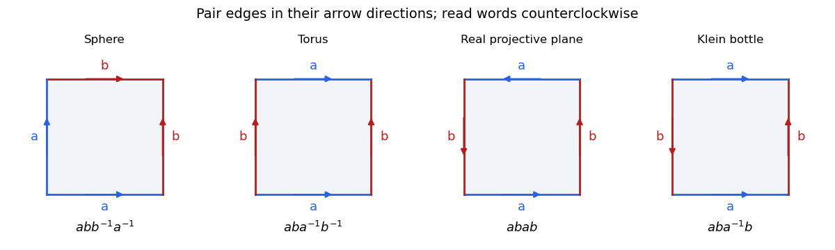
Start with a polygonal disk and pair all its sides, specifying for each pair a homeomorphism matching endpoints. Arrow labels encode whether each occurrence is traversed with or against its assigned direction. Form the quotient topology using those identifications and no extra identifications in the interior. Matched edge interior points have disk neighbourhoods formed from two half-disks; the corner sectors around each identified vertex form a circular link. The quotient is therefore a closed surface. A boundary word records each edge label exactly twice. Its endpoint identifications determine the vertex count, while its signs determine orientability. This encoding is distinct from treating a side-paired polygon as an abstract simplicial complex; a compatible subdivision is needed for a simplicial triangulation.

For a polygonal schema with all its sides paired and two same-direction occurrences of an edge label $x$, the words $xAxB$, $xx{A}^{-1}B$, and $A^{-1}xxB$ describe homeomorphic quotient spaces. Here inversion of a string reverses its order and inverts each letter. Cut from the start of the first $x$ side to the start of the second, using a diagonal $d$. The pieces have boundary words $xA{d}^{-1}$ and $dxB$. Gluing the old $x$ sides gives outside word $A{d}^{-1}{d}^{-1}{B}^{-1}$; reversing the whole boundary and choosing a new starting point gives $dd{A}^{-1}B$. Alternatively cut from the end of the first $x$ side to the end of the second. The pieces are $xdB$ and $Ax{d}^{-1}$, and gluing their old $x$ sides gives $dB{A}^{-1}d$, cyclically $A^{-1}ddB$. Renaming the new paired side gives both asserted forms. These are actual cutting and gluing homeomorphisms, so they preserve all the other side identifications as well as the Euler characteristic.

Given a cyclic-factor subnormal series $1=G_0⊴\cdots ⊴G_n=G$ and $H\le G$, intersect each term with $H$. The induced map $(H\cap G_{i+1})/(H\cap G_i)\to G_{i+1}/G_i$ is injective. Since every subgroup of a cyclic group is cyclic, the intersection chain is again a cyclic-factor subnormal series, after removing repetitions. Hence $H$ is a polycyclic group. In particular, every subgroup is finitely generated.

If a group has a cyclic-factor subnormal series of length $n$, choose one lift of a generator of each nontrivial factor. Induction gives $G_i=⟨G_{i-1},g_i⟩$, so the chosen lifts generate $G$. Thus at most $n$ generators are needed. Applying this to the intersection chain in subgroups of polycyclic groups are polycyclic bounds the number of generators of every subgroup by the same series length.

Both colour counts tend to infinity almost surely. For example, $X_n\ge B_0/(m+n)$, and independent events $U_{n+1}\le B_0/[2(n+1)]$ occur infinitely often by the Borel-Cantelli second lemma, forcing infinitely many blue additions.

The martingale increment formula gives $\mathbb{E}[(X_{k+1}-X_k{)}^2\mid {\mathcal{F}}_k]\le X_k/(m+k+1{)}^2$. Conditional orthogonality of later increments and $\mathbb{E}[X_k\mid {\mathcal{F}}_n]=X_n$ implyOn $X_{\infty }=0$ the squared difference is $X_n^2$, so its conditional probability is at most $1/[(m+n)X_n]=1/B_n\to 0$. Dominated convergence proves zero probability of that endpoint. The symmetric argument for red excludes $X_{\infty }=1$. No explicit beta law is needed for this proof.

An angular polarimeter associated with Jean-Baptiste Biot, measuring the rotation produced by a sugar solution of known optical path length. The original form used a black-glass polarizing mirror and a calcite analyser; it should not be conflated with a later quartz-wedge compensating instrument.^[ref]

For the one-dimensional Sobolev representative with $v(c)=0$, the fundamental theorem of calculus gives $v(x)=-{\int }_x^c{v}^{\prime }(t)dt$. The Cauchy-Schwarz inequality then gives $|v(x){|}^2\le (c-x)\Vert v^{\prime }{\Vert }_2^2$. Integrating proves the displayed, generally nonoptimal Poincaré inequality. In particular $\Vert v{\Vert }_{H^1}^2\le [1+(c-b{)}^2/2]\Vert v^{\prime }{\Vert }_2^2$. Only one endpoint must be fixed, which is useful for mixed boundary conditions and for controlling a negative potential.

The displayed scalar stress potential automatically satisfies the two in-plane static momentum equations without body force, because the mixed third derivatives cancel. For homogeneous isotropic linear elasticity, strain compatibility further makes $A$ biharmonic. Since stresses depend only on second derivatives, $A$ is unique only up to $ax+by+c$ on a connected domain. Conversely a function with all second derivatives zero is affine, proving that this is exactly the gauge freedom. It does not license adding an arbitrary biharmonic function, which generally changes stress.

For an isotropic elastic annulus $a<r<b$ with internal excess pressure $P$ and zero outer gauge pressure, radial equilibrium gives $u=Cr+D/r$. Its stress tensor has ${\tau }_{rr}=2(\lambda +\mu )C-2\mu D/r^2$ and ${\tau }_{\theta \theta }=2(\lambda +\mu )C+2\mu D/r^2$. Enforcing ${\tau }_{rr}(a)=-P$, ${\tau }_{rr}(b)=0$ gives $2\mu D=P{a}^2{b}^2/(b^2-a^2)$, so the maximum difference occurs at the bore and equals the displayed expression. Once an appropriate yield criterion is reached, stress must be related to elastic strain while total strain includes a plastic contribution. The elastic formula alone cannot describe further irreversible deformation.