
A tractrix is a plane curve whose tangent segment from the point of contact to a fixed axis has constant length. For segment length one and a positive acute tangent angle , its height is . The slope relation gives . Integrating yields the displayed axial coordinate up to an additive constant. Conversely these coordinates have the required slope, and their tangent intercept is at distance . Rotating this profile about its axis gives a tractoid.
A transported planar potential dipole follows the surrounding regular velocity, so its position satisfies the displayed equation after its own singular term is removed. The conjugation comes from the convention . Reflected image parameters are held fixed when taking the spatial derivative, then evaluated at the instantaneous dipole position.
For a unit circular wall, the Milne-Thomson circle theorem gives image potential and therefore . For a horizontal straight wall the image is , giving . For the line , reflected conjugation gives image and hence . In each case the image lies outside the fluid region and makes the wall a streamline; differentiation of the regular image proves the motion formula. Several compatible straight-wall reflections can be summed before the same operation is applied.
For the autonomous differential equation , the displayed family stays at until time and then decreases below it. Here . Direct differentiation verifies the equation on each side; since , the derivative tends to zero at departure, making the joined function continuously differentiable. Distinct departure times give different solutions from the same equilibrium initial condition. The ratio is unbounded, so the local Lipschitz continuity hypothesis of the Picard-Lindelöf theorem fails.
A solution starting above reaches it in finite time. It can then use any of these continuations. For , , and initial value , arrival occurs at time two; departure at gives afterwards. Waiting-time solutions of a sublinear Bernoulli equation give a related mechanism for departures in the opposite direction.
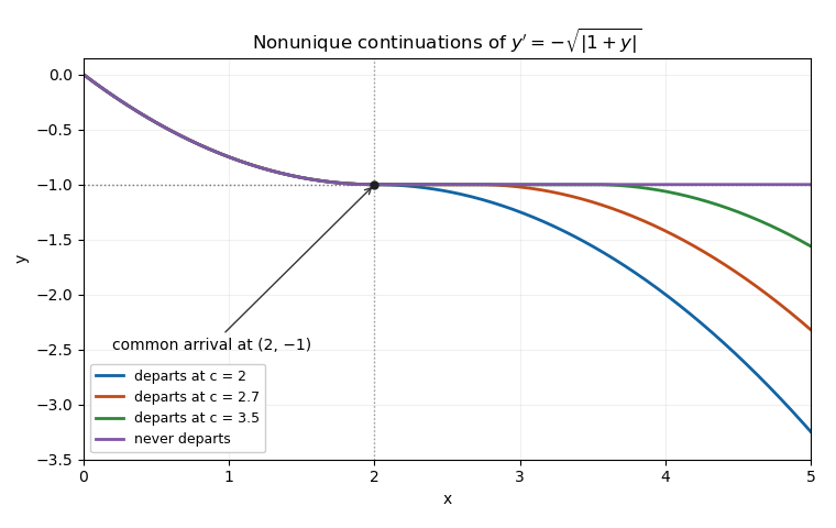
Different waiting-time continuations at a non-Lipschitz equilibrium share the same earlier trajectory
. Details. 
Suppose is continuous and Lipschitz in its state variable on a closed cylinder , , with bounds and Lipschitz constant . On a smaller interval of radius , the displayed Picard operator maps continuous curves in that closed ball into itself when , and it is a contraction mapping in the supremum norm when . This function space is complete because it is a closed subset of a Banach space of continuous vector-valued functions. The contraction mapping theorem gives a unique fixed point, and the fundamental theorem of calculus makes it a solution of the ordinary differential equation. Choosing also prevents any solution with the same initial data from first exiting the cylinder during that interval.
A coefficient that vanishes at the initial time can hide failure of the uniform Lipschitz condition required for an initial value problem. For , the map is identically zero. But every rectangle of positive widths around contains some , andNo Lipschitz constant works uniformly on the rectangle. Actual uniqueness also fails: and are distinct differentiable solutions with initial value zero. Substitution gives for the second solution. A condition at the single initial time cannot replace control on a neighbourhood.
For the ordinary differential equation through , consider a symmetric existence rectangle , . Its maximum slope bound is . The condition becomes . Differentiating shows its maximum occurs at , givingThis is the largest interval guaranteed by this particular centered-rectangle criterion. Direct separation of variables instead gives on the maximal real interval . The comparison shows the difference between a sufficient local existence theorem and the actual continuation interval. The endpoint obstruction is the zero of the denominator at .
The source of the medicinal seed called Calabar bean.
Explanation of bulk assimilate transport from source to sink through hydrostatic pressure differences associated with solute loading and unloading.
A periodic phase response function describes the first-order phase shift produced by a perturbation along a limit cycle. With period-one orbit , choose the periodic adjoint solution normalized by . The Fredholm solvability condition then projects forcing to . For voltage-difference coupling, the averaged interaction is .
Linearizing weakly coupled locked phases gives , where is the directed graph Laplacian. Multiplying by a normalized left null vector eliminates coupling and gives the displayed weighted frequency. In a balanced network, including symmetric reciprocal coupling, and the frequency is the arithmetic mean. A zero diagonal in the coupling matrix alone does not imply balance. For two directed weights , the weights are .
The Perron's formula kernel integrates to , giving the smoothed sum as an integral of . For each fixed height , a zero-free rectangle permits shifting the central contour to a real part below one; its vertical contribution is , and its horizontal contributions are when the original real part is . A bound for bounds the remaining tails by . Letting grow first and afterward proves the displayed cancellation, without uniform estimates to the left of one.
With , periodic functions have the displayed convolution identity for every real . Apply the polarized Parseval identity to and ; a change of variable gives the latter function's pairing with . The Cauchy-Schwarz inequality bounds the sum of absolute coefficient products by , so the resulting series converges absolutely and uniformly. This proves continuity of the convolution even though neither original Fourier series need converge pointwise.
A rank-two period lattice stable under multiplication by is, up to nonzero complex scaling, . Choose a shortest nonzero period . Every complex number lies within of a Gaussian integer, so for any , subtraction of a suitable leaves a shorter period and hence zero. This proves .
Similarly, stability under a primitive cube root gives . The triangular lattice has covering radius , so the same shortest-period argument applies. Stability under a primitive sixth root is equivalent, since . These facts identify complex tori with automorphisms fixing their origin of orders four and three or six, respectively.
For disjoint closed sets in a subspace , their ambient closures satisfy . In a perfectly normal space choose continuous functions with exact zero sets . The function is continuous on , which contains , and separates . Disjoint inverse images of endpoint neighborhoods give normality of .
For , the third forward difference annihilates polynomials of degree at most two. Its Peano kernel is for , extended by zero outside that interval. It is times the quadratic cardinal B-spline evaluated at , is positive on , and has integral . The Peano kernel theorem therefore represents as a positive weighted average of the third derivative: for some interior when that derivative is continuous. The kernel is the smooth error weight hidden inside a discrete difference.
The Peano kernel theorem writes a derivative-based error functional as , so its bound in the displayed derivative seminorm is at most the L1 norm of the kernel. This is the sharp constant: continuous derivatives can approximate the sign of in the weighted integral, and integrating them times produces admissible test functions. If has one sign, a constant th derivative already attains equality; in particular . This provides a direct exact check on proposed error constants before estimating individual polynomial pieces.
An infinite path in a transition system represented by a finite prefix followed by infinite repetition of a nonempty finite loop. If stored positions are and , the represented sequence is . The linear temporal logic condition holds exactly when occurs on the repeated part, and holds exactly when holds everywhere on that part.
There are unlisted articles, also show them or only show them.