A nonzero vector is an eigenvector of a linear operator when for some eigenvalue . For a real vector space and , the line through is preserved: the image can point forward or backward, but cannot turn away from that line. When , the image is zero and has no direction. The zero vector is excluded because it satisfies the equation for every scalar and identifies no special direction.
Every nonzero scalar multiple of an eigenvector is an eigenvector for the same eigenvalue, since . Thus there is usually no preferred length or sign; choosing a unit vector is a convenient normalization. Eigenvectors for a fixed eigenvalue, together with zero, form its eigenspace.
For a fully computed example, consider the real symmetric matrixIts characteristic polynomial isFor , gives , so is an eigenvector. For , gives , so is an eigenvector. Direct multiplication checks both:The map stretches the line threefold and fixes the line pointwise. These eigenvectors are orthogonal because ; dividing each by gives an orthonormal basis. A general vector turns because its components along these two lines receive different scalings. For example, maps to and is not an eigenvector.
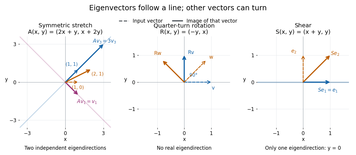
A contrasting example is the planar rotation through degrees:Every nonzero real vector turns to a perpendicular direction, so there are no real eigenvectors. Its characteristic polynomial is , which has no real roots. Over the complex numbers, however, and . The same matrix therefore has an eigenbasis in even though it has none in : the choice of field matters.
If , the smallest operator-norm perturbation that makes an exact eigenpair has norm . One such rank-one perturbation is
Edge-isoperimetric inequality in the discrete cube by  Codex 0 Created 2026-09-24 Updated 2026-10-14
For ,
Equivalently, spans at most cube edges. Induction on the dimension and concavity of binary entropy prove the inequality.
On a finite measure space, a positive functional defines the finite measure . The Radon-Nikodym theorem gives with . The boundand - norm duality imply , after which density extends the integral representation to every .
The double slice genus is the smallest genus of an unknotted closed orientable surface in whose transverse equatorial cross-section is .
If is a Sylow subgroup of a finite group and , some intersection is a Sylow subgroup of . Otherwise every double-coset sizewould be divisible by a larger power of than , as would their sum .
A discrete-time martingale with converges almost surely to an integrable random variable. If the martingale is uniformly integrable, convergence also holds in .
This is one of Doob's martingale convergence theorems; uniform integrability upgrades almost-sure convergence to convergence in mean.
Drag on a two-dimensional circular bubble from outer-flow dissipation by Codex 0 Created 2026-09-24 Updated 2026-09-24
Codex 0 Created 2026-09-24 Updated 2026-09-24For the zero-circulation flow around a circle, . Integration over the exterior plane gives dissipation per unit axial length and hence drag per unit length.
This tensor is a local derivative of the displacement field; it enters the deformation gradient and strain measures.
For a dispersion relation , the phase velocity is and the group velocity is . For the Klein-Gordon relation at ,
For a normal mode proportional to , the real part is its exponential growth rate. A positive growth rate signals linear instability.
Discrete sine transform from a sign-modulated discrete cosine transform by Codex 0 Created 2026-09-24 Updated 2026-10-14
Codex 0 Created 2026-09-24 Updated 2026-10-14For , a Poisson random variable has probability mass functionThe exponential function series verifies normalization. At , define with certainty. The equality of mean and variance is a distinguishing model property, though it does not by itself characterize the law.
When counting events in a homogeneous Poisson process, distinguish its rate from the distribution parameter: an interval of duration has . A rate measured per minute times a duration measured in minutes gives a dimensionless expected count. This process assumes independent increments, a constant rate, and a negligible chance of multiple events relative to interval length in a sufficiently short interval. A rate alone does not establish a Poisson distribution. See Bertsekas and Tsitsiklis, chapter 6 summary, pages 46-47.
For a constructed arrival model with events per minute over minutes, . The mean and variance are both three, andThe probability of at least one event is . These results describe the specified process, not every arrival mechanism with the same average rate.
The Poisson limit theorem, often called the law of rare events, connects this law to the binomial distribution. Keep fixed and let for integers . For each fixed nonnegative integer and sufficiently large ,There are more opportunities, each less likely to succeed, while the mean stays and the variance approaches . For , the probability of three successes is at , at , and at , approaching the Poisson distribution value .
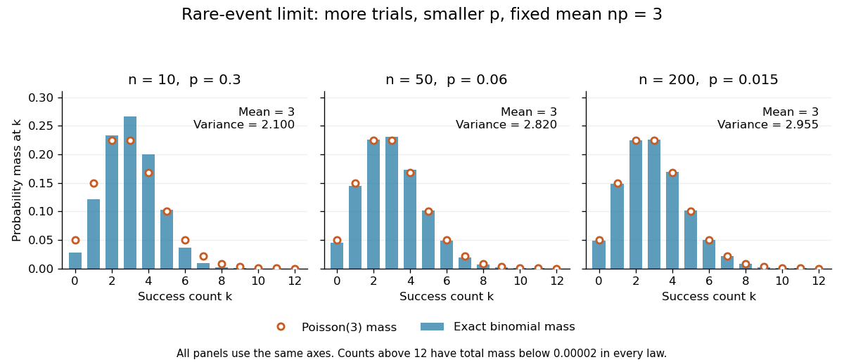
The panels show the same count scale and the same Poisson distribution reference. At , is not especially small and the difference is visible. No universal trial-count cutoff guarantees an adequate approximation for every event.
The independence assumption matters even when every success is rare. For , if all indicator random variables equal one shared Bernoulli random variable of parameter , their sum is zero with probability and with probability . Its mean is three, yet its zero-count probability tends to one, not . Some dependent counts still admit approximation through the Stein-Chen method, but this requires additional control of dependence.
For historical orientation, the BnF records Poisson's original probability treatise, Recherches sur la probabilité des jugements, as published in Paris in 1837. This bibliographic fact alone does not establish when the modern distribution terminology arose. See BnF record of Poisson's 1837 treatise.
A multinomial distribution describes category counts from independent trials, each choosing exactly one of categories with the same probabilities . Require to be an integer, , and . If counts the trials in category , then andThe are integers, and the mass is zero for other count patterns. A category with has count zero almost surely, with in this formula. For a specified ordered trial sequence, independence gives the product of numbers ; the multinomial coefficient counts the different sequences with that same count pattern.
For four trials with category probabilities , the count pattern can occur in orders, each of probability . Thus its total probability is . This is a constructed independent-trial example, distinct from drawing four objects without replacement from a ten-object population of composition , where the multivariate hypergeometric distribution gives .
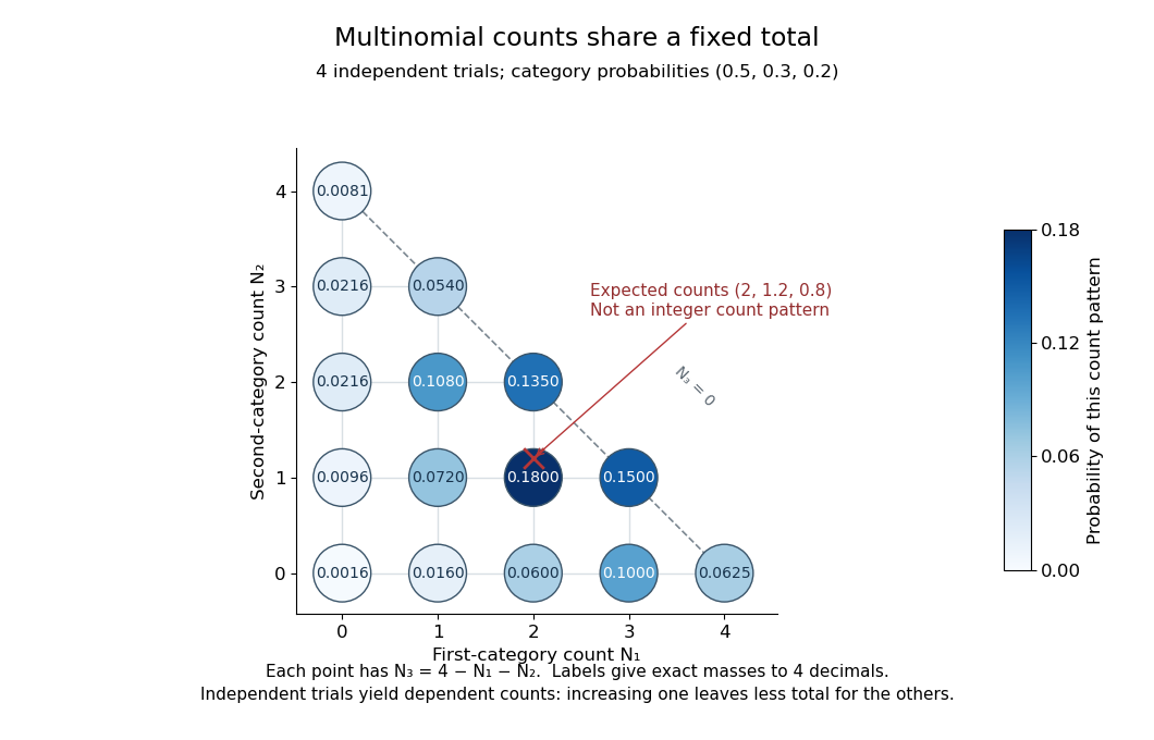
Three category counts from four independent trials: every point fixes the third count through the total
. Details. The diagram shows all fifteen possible count patterns. Coordinates determine ; the triangle is a constraint on integer counts, not a continuous probability density. The mode is , where the probability mass function is largest, but the expected values are not a possible count pattern.
Each single count has a binomial distribution, because recording category versus all other categories reduces every trial to a Bernoulli trial. Consequently,These statements about the joint count model are summarized in Aditya Guntuboyina's lecture notes.[ref]
https://stat238.berkeley.edu/spring-2026/lecturetwelve238spring2026/. Guntuboyina, Berkeley STAT 238, lecture 12: multinomial distribution
Independent trials do not make the resulting counts independent random variables. Within one trial the indicator random variables for two distinct categories cannot both equal one, so their product is zero and their covariance is . Summing over independent trials gives . In the four-trial example, the variances are and the pairwise covariances are . Knowing that all four trials were in the first category fixes the other two counts at zero.
The attraction is that one formula describes any fixed-total list of category counts while preserving the constraint that they add up to . It underlies multinomial likelihood calculations and uniform balls-in-bins allocation. The multinomial aggregation rule lets us merge categories without leaving this family of probability distributions. Allowing independent category counts with an unfixed total instead leads to a different model, related through Poisson-multinomial conditioning.
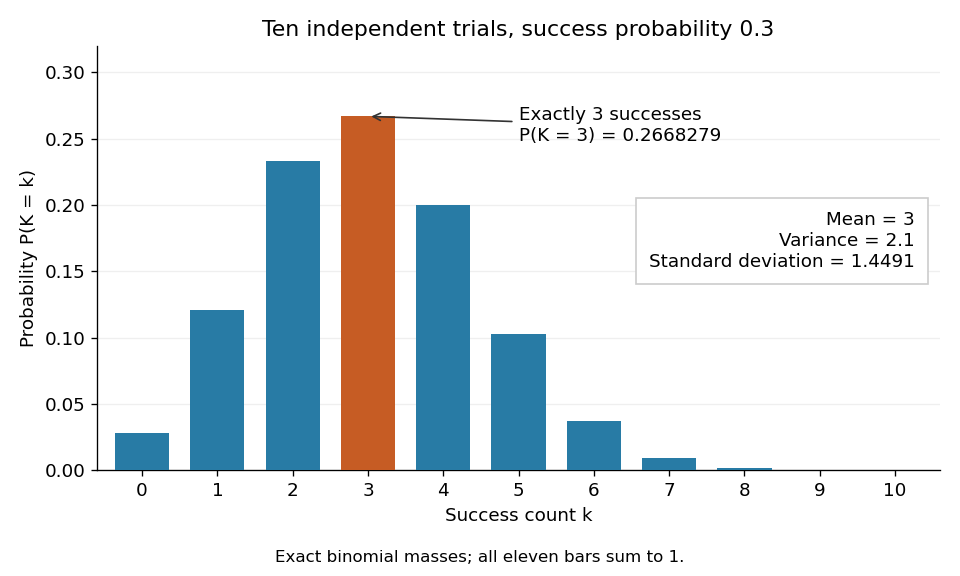
The binomial distribution counts successes in a fixed number of independent Bernoulli trials with common success probability . Equivalently,Here is a nonnegative integer and . The binomial coefficient counts placements of the successes; each particular arrangement has probability . The binomial theorem makes the masses sum to . At all mass is at zero, and at all mass is at ; these endpoint laws can be read directly without interpreting .
The linearity of expectation and addition of variances for independent random variables giveThe fixed trial count, common success probability, and joint independence are substantive model assumptions. Sampling uniformly without replacement from a finite population instead leads to a hypergeometric distribution. Independent trials with different success probabilities generally give a Poisson binomial distribution. Common marginal success probabilities alone are insufficient: if all ten indicators equal the same Bernoulli random variable with , their sum is zero with probability or ten with probability . Its mean is still three, but its variance is . The standard construction is given in Penn State STAT 504, binomial distribution.
For an exact constructed example, let each of ten independent trials choose uniformly from ten labelled tokens, with replacement, and mark three tokens as successes. Then and . Exactly three successes have probabilityThe mean is , the variance is , and the standard deviation is . Zero successes have probability , so at least one success has probability . A single count calculation replaces enumeration of all equally likely token sequences.


There are unlisted articles, also show them or only show them.