A magnetic field is a vector field whose local value determines the magnetic part of the Lorentz force on a body with electric charge and velocity . In SI units,where is the speed, , and is the angle between the velocity and the magnetic field. The cross product makes a nonzero magnetic force perpendicular to both the velocity and the magnetic field. The right-hand rule gives its direction for positive electric charge; negative electric charge reverses it. [ref].
The SI unit of magnetic field is the tesla:For a stipulated example in SI units, take electric charge , velocity , and magnetic field . The cross product gives magnetic force . With the same speed directed along , the magnetic force is zero: motion parallel to a magnetic field produces no magnetic acceleration.
Magnetic field lines visualize the direction of a magnetic field by being tangent to it at each point. They are not generally the path of a body with electric charge: in a uniform magnetic field along , the magnetic field lines are straight while transverse velocity produces circular motion, and adding parallel velocity produces helical motion in a uniform magnetic field. The worked Lorentz force example below illustrates this distinction.
A magnetic field need not be static. Magnetostatics is the restricted case with no dependence on time; an electromagnetic wave has changing electric field and magnetic field even in vacuum. A changing magnetic field is coupled to the electric field through Faraday's law of induction. [ref]
https://www.feynmanlectures.caltech.edu/II_20.html. Feynman lectures, II.20: electromagnetic waves in free space
. The useful separation is between local bending, described by the Lorentz force, and the amount of magnetic field crossing a surface, described by magnetic flux.Electric charge is an additive, signed property of matter that determines its coupling to the electromagnetic field. Write a particle's electric charge as , or a collection's total electric charge as ; the SI unit is the coulomb, . A stationary test particle in an electric field experiences electric force , while motion adds the magnetic part of the Lorentz force. Electric charge both produces an electric field and determines the response to one. For two stationary point particles in vacuum, Coulomb's law makes like signs repel and opposite signs attract. The choice of which sign to call positive is a convention, used consistently: protons carry and electrons carry , where is the elementary charge. [ref]
https://www.feynmanlectures.caltech.edu/II_01.html. Feynman, Leighton and Sands, II.1: electrical forces, fields and the Lorentz force
.Additivity means adding signed electric charges, rather than their magnitudes:for ordinary matter containing protons, electrons, and electrically neutral neutrons. A toy collection with seven protons and ten electrons has , however much neutral material accompanies it. Charge neutrality means ; it does not mean an absence of charged constituents. Nor does it guarantee an absence of electric force: the spatial arrangement of positive and negative electric charges matters, as illustrated by an electric dipole. This makes a tiny imbalance in an otherwise nearly neutral object physically important. [ref]
https://www.feynmanlectures.caltech.edu/II_01.html#Ch1-S1. Feynman, Leighton and Sands, II.1.1: neutrality, imbalance and residual electrical forces
.Charge conservation states that a collection closed to transport of electric charge keeps its total signed . If electrons move from object A to object B without other exchange, then and ; the sum is unchanged. The amount of positive electric charge alone need not be conserved: creation of an electron and a Positron adds opposite electric charges with zero sum. These bookkeeping rules let us distinguish separation or transport of electric charge from creation of net electric charge. [ref]
https://www.feynmanlectures.caltech.edu/I_04.html#Ch4-S4. Feynman, Leighton and Sands, I.4.4: conservation of net charge
.A simple motivating experiment uses two charge-producing paddles, a conducting pail on an insulating support, a grounded outer shield and a high-input-impedance electrometer. Zero the pail, then isolate it. Rub the initially neutral paddles together, keeping their charged surfaces away from other objects. Lower each deeply into the pail without touching: the electrometer gives opposite signs. Inserting both together tests cancellation. For a separate contact test, insert one charged paddle without touching and withdraw it: the reading returns to zero. Repeat after zeroing, this time touching the inner wall before withdrawal: a residual reading shows transfer of electric charge. Zero the pail and reinsert the paddle to test how much electric charge remains on it. PASCO describes these procedures in Basic Electrostatics System manual, demonstrations 1A and 1B, printed pp. 13–16.
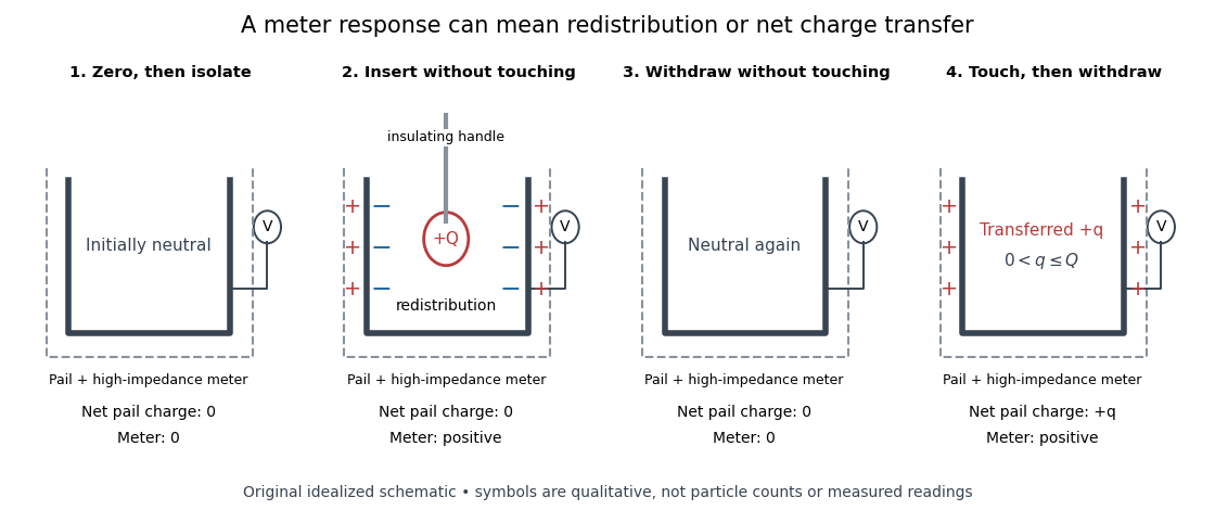
Electric charge redistribution versus transfer in a conducting pail
. Original qualitative schematic for a positively charged inserted object. Without contact, electrostatic induction separates negative inner-surface and positive outer-surface electric charges, while the pail's total remains zero. Contact can leave net positive electric charge after withdrawal. Symbols are not particle counts; no measured readings are plotted. Source. Details.
The crucial control is withdrawal without contact: a response during insertion can come from electrostatic induction, which redistributes the pail's existing electric charge. In the fixed-geometry approximation, the electrometer measures electric potential difference proportional to enclosed electric charge, with conversion set by effective capacitance; a voltage reading is not already a measurement in coulombs. Opposite readings and their cancellation test additivity and charge conservation within resolution. Leakage or accidental contact spoils that interpretation, and contact need not transfer all the paddle's electric charge. This macroscopic experiment cannot resolve elementary charge steps: that requires the much smaller particles of the oil drop experiment.
The right-hand rule fixes the orientation of a cross product and relates the circulation direction of an electric current to the direction of its magnetic field.
After reducing conserved cyclic momenta, an equilibrium at a strict local minimum of the resulting effective potential is stable in the reduced one-degree-of-freedom dynamics.
A Lyapunov function near an equilibrium is continuously differentiable, satisfies and away from , and has orbital derivative
Equilibrium of an autonomous differential equation by  Codex 0 Created 2026-09-24 Updated 2026-10-03
An equilibrium is a state where the autonomous vector field vanishes.
An equilibrium is unstable when arbitrarily small perturbations can move trajectories away from it.
Fixed point stability for an autonomous differential equation by Codex 0 Created 2026-09-24 Updated 2026-09-24
Codex 0 Created 2026-09-24 Updated 2026-09-24A Floquet multiplier is an eigenvalue of a one-period linear evolution map. For a homogeneous linear differential equation with continuous coefficients of period , this map is the monodromy matrix of a periodic linear system . If for a nonzero eigenvector , the associated solution of a differential equation with satisfies . Its exponential rate is , the corresponding Floquet growth rate. A Floquet multiplier equal to one gives a -periodic solution in that eigenvector direction; a nontrivial Jordan block at a unit-modulus Floquet multiplier can still produce polynomial growth.
For a nonlinear periodic orbit, the Floquet multipliers are eigenvalues of the one-period map of its variational equation. A nonconstant periodic orbit of a smooth autonomous differential equation has a Floquet multiplier equal to one in its tangent direction: differentiating the solution of a differential equation with respect to its starting phase gives a periodic solution of the variational equation. The derivative of a transverse Poincaré map removes this phase direction and retains the transverse Floquet multipliers. Transverse Floquet multipliers strictly inside the unit circle give local attraction, while one outside gives instability; a transverse Floquet multiplier on the unit circle requires further analysis. For a planar periodic orbit, the transverse Floquet multiplier is given by the divergence test for a planar periodic orbit.
A periodic orbit is a nonconstant trajectory that returns to its initial state after some least positive period.
The omega-limit set of a trajectory consists of the points approached along sequences of times tending to positive infinity. For a bounded continuous flow it is nonempty, compact, connected, and invariant.
An autonomous planar system is an ordinary differential equationwhose vector field does not depend explicitly on time.
At a hyperbolic fixed point, stable and unstable manifolds are tangent to the corresponding eigenspaces. Power-series coefficients follow from graph invariance.
There are unlisted articles, also show them or only show them.