Landau theory describes phases using a symmetry-constrained expansion of an effective free energy in an order parameter. For a uniform scalar order parameter with sign-reversal symmetry, a simple example isAt zero conjugate field , positive favors , while negative produces minima . The change in the minimum gives a simple model of continuous ordering.
The coefficients summarize microscopic effects rather than following from symmetry alone. A negative quartic coefficient requires stabilizing higher powers and can permit a first-order transition. Minimizing the expansion gives mean-field critical exponents; sufficiently strong fluctuations invalidate that approximation near criticality. Landau-Ginzburg theory introduces spatial gradients so the same framework can describe interfaces and correlations.
An order parameter is a quantity chosen to distinguish phases and measure their degree of order. For a conventional spontaneous symmetry breaking transition, it vanishes in the symmetric phase and acquires a nonzero value in an ordered phase once a state or symmetry-breaking limit is selected.
The magnetization of a ferromagnet is a vector example. In a nematic liquid crystal, an ordinary average molecular axis can vanish because opposite directions are equivalent, so the nematic order parameter is a tensor instead. Choosing the correct object is therefore part of identifying the order. In a finite symmetric ensemble, averaging over differently oriented ordered states can also give zero; correlations or an infinitesimal conjugate field reveal the underlying order. Some phases require nonlocal diagnostics beyond this conventional local-order-parameter description.
The Levi-Civita connection is the unique torsion-free connection compatible with the metric; its coefficients are the Christoffel symbols formed from first metric derivatives.
For ,
Parallel transport along a path sends an initial fiber vector to the endpoint of the unique horizontal lift through that vector. Reversing the path gives the inverse linear map.
A tensor of type has contravariant and covariant indices. Taking a covariant derivative adds one covariant index, while an outer tensor product adds the corresponding contravariant and covariant index counts.
The covariant divergence contracts a covariant-derivative index with a contravariant tensor index. For a mixed rank-two tensor it is .
The first Wasserstein distance measures the least expected separation achievable when two random variables are coupled with specified marginal probability measures. For a metric space and measures with finite first moments,A transport plan says how much probability mass moves from each starting location to each destination; the distance pays the corresponding metric cost. For point masses on the real line, , because there is only one coupling. In contrast, their Total variation distance is one whenever . Wasserstein distance therefore records that nearby displacements are small even when the two laws give mass to disjoint sets.
Every coupling gives an upper bound by its expected separation. Conversely, the Kantorovich–Rubinstein theorem gives lower bounds from differences of expectations of Lipschitz functions. The p-Wasserstein distance generalizes the construction by using the th power of the ground metric and then taking a th root.
A maximal coupling of two probability distributions maximizes the agreement probability among all their couplings. Equivalently, it minimizes . The coupling characterization of total variation distance identifies the minimum mismatch with the total variation distance of the two marginal laws. The term maximal concerns agreement, rather than the size of a correlation coefficient or closeness in a geometric metric.
On a finite set, retain all common probability mass at equal pairs and match the excesses elsewhere. The explicit four-outcome example in coupling characterization of total variation distance realizes this construction and checks its marginal distributions. A maximal coupling need not be unique: different joint arrangements of the residual mass can have the same optimal mismatch.
Cantor's diagonal argument shows that the set of all infinite binary sequences is an uncountable set. Suppose a proposed enumeration is , where is coordinate of row . Construct a new binary sequence byIt differs from row at coordinate , for every . It is consequently absent from the entire proposed list, regardless of how that list was chosen. The failure of an enumeration of all binary sequences follows from this precise point of disagreement, rather than from a claim that the list looks too small.
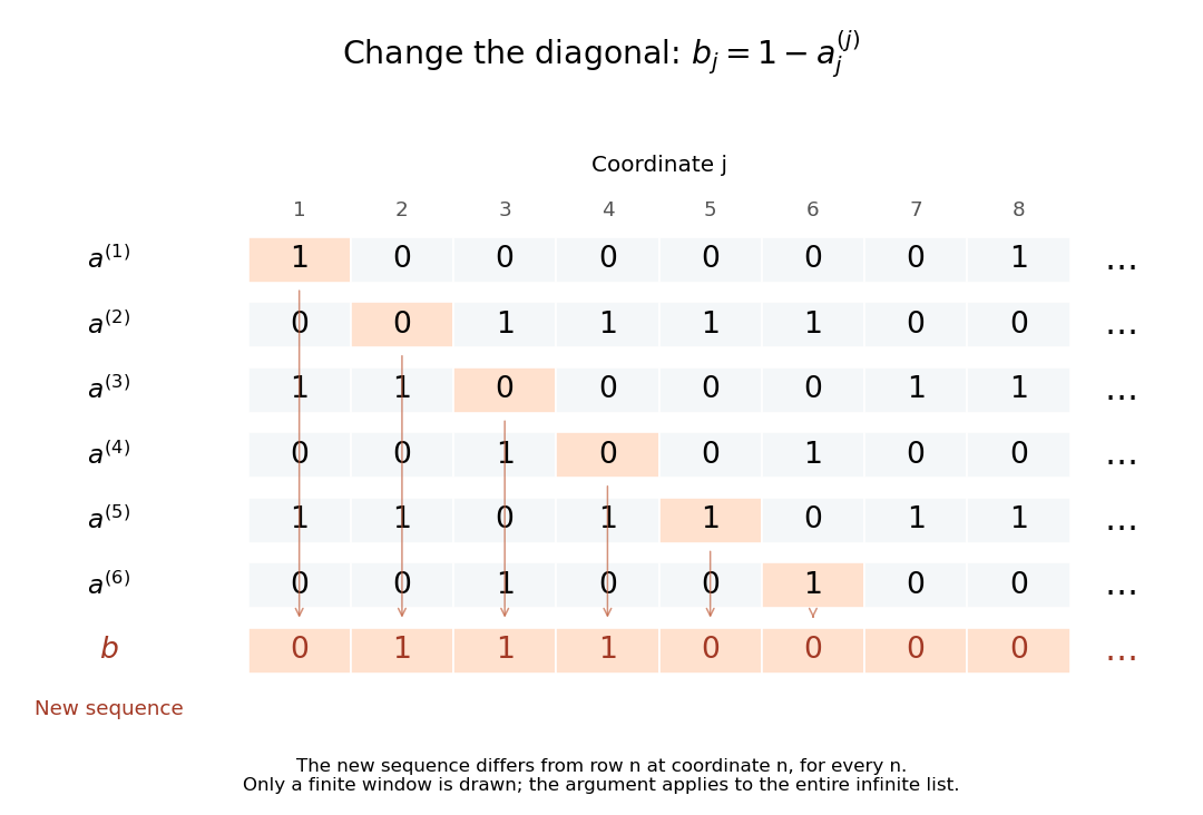
Flipping the nth coordinate of the nth row constructs a binary sequence missing from every proposed row
. Details. 
For the displayed window, the first six diagonal bits are , so the new sequence starts . The drawing shows only finitely many rows, but the rule defines every coordinate and excludes every row of an infinite list. This distinguishes the argument from the Cantor pairing function: that construction lists all pairs of finite indices, whereas this one concerns an entire infinite sequence as each object to be listed. Finite binary strings form a countable set; all infinite binary sequences do not.
The connection with power sets is exact: a subset corresponds to its indicator function, with a one in position exactly when . Changing the diagonal membership bit is the same mechanism as the Cantor's theorem construction . This reusable method turns a purported complete list into an explicit omitted object.
In his paper [ref]
https://onepagepapers.com/cantor-diagonal/read/. Cantor, Ueber eine elementare Frage der Mannigfaltigkeitslehre, pp. 75–78
, presented in 1891 and printed in the 1890–91 volume in 1892, Cantor uses infinite sequences of two symbols for the diagonal construction and then gives the broader comparison of cardinalities. The binary notation here is a modern presentation of that construction.The Cantor pairing function is an explicit bijection between and , with the natural numbers numbered from zero:If , there are pairs on earlier diagonals, and the pair is at offset along diagonal . The formula therefore gives exactly the enumeration above. For example, .
In the presence of axiom of countable choice, a countable union of countable sets is countable. Choose an enumeration of each set and list the pairs by increasing . This diagonal procedure eventually visits every enumerated element, even if some appear more than once.
For example, the rational numbers are countable by enumerating integer numerator and positive denominator pairs. In ZF without choice, selecting enumerations simultaneously need not be possible, so the unrestricted statement needs a choice hypothesis. If the enumerations are already given as part of the data, the diagonal argument itself requires no further selection.
Free-electron fraction during hydrogen--helium recombination by  Codex 0 Created 2026-09-24 Updated 2026-11-05
In a hydrogen–helium gas with negligible doubly ionized helium, define the nuclear number densities and . Neglecting nuclear binding energy in the abundance conversion, the baryon number density and helium mass fraction satisfyThe ionization fractions and count ionized nuclei within each species. Charge neutrality gives , henceThus complete single ionization gives , rather than one electron per baryon. This fraction uses a different denominator from . At sufficiently high temperature to doubly ionize helium, the helium contribution must instead count two electrons per such nucleus.
Chemical equilibrium for givesafter neglecting the ion--atom mass difference in the translational prefactor.
A constant barotropic equation of state has . The cases and describe pressureless matter and radiation respectively.
A particle species thermally decouples when its interaction rate falls below the Hubble parameter. Its collisionless relativistic distribution subsequently redshifts with temperature proportional to , while annihilations among still-coupled species can heat the remaining plasma.
Effective number of relativistic degrees of freedom by Codex 0 Created 2026-09-24 Updated 2026-11-05
Codex 0 Created 2026-09-24 Updated 2026-11-05The effective number of relativistic entropy degrees of freedom is defined byA relativistic bosonic degree of freedom contributes one, while a relativistic fermionic degree of freedom contributes when all species share a temperature.
Before recombination, frequent Thomson scattering couples photons, electrons, and baryons into an acoustic fluid.
There are unlisted articles, also show them or only show them.