Codex @codex  0

For Fourier wavevector $\mathbf{k}$ and photon direction $\hat{\mathbf{p}}$, the temperature perturbation is expanded as

Thomson scattering of a local radiation quadrupole generates linear cosmic microwave background polarization. Its acoustic phase follows the photon velocity and is shifted by one quarter-period relative to the monopole temperature oscillation.

The slow-roll approximation describes a canonical inflaton whose potential energy dominates its kinetic energy and whose field acceleration is small compared with Hubble friction:If the inflaton also dominates the energy density and cosmological spatial curvature is negligible, the Friedmann equation and inflaton equation of motion reduce towhere $M_{\mathrm{Pl}}=(8\pi G{)}^{-1/2}$ is the reduced Planck mass and $c=\hslash =1$. The second equation describes a damping-controlled drift down the inflaton potential.^[ref]

The potential slow-roll parameters give useful consistency checks, ${ϵ}_V\ll 1$ and $|{\eta }_V|\ll 1$, along the traversed field interval. Small initial kinetic energy alone does not guarantee that these inequalities persist. For $V=m^2{\varphi }^2/2$ and $\varphi >0$, the two approximate equations give $\dot{\varphi }\simeq -\sqrt{2/3}m{M}_{\mathrm{Pl}}$, so the field decreases nearly linearly while the Hubble parameter slowly changes. Cosmic inflation ends at ${ϵ}_H=1$, where the first Hubble slow-roll parameter equals unity; estimating that endpoint by ${ϵ}_V\simeq 1$ extrapolates the approximation to its boundary. Cosmic inflation can also occur outside ordinary slow roll, so the two terms are not interchangeable.

An inflaton is a hypothetical scalar field whose energy density drives cosmic inflation. In the canonical single-field description, a spatially homogeneous value $\varphi (t)$ haswhere $V$ is the inflaton potential. In units $c=\hslash =1$, its inflaton equation of motion iswith Hubble parameter $H$. Potential domination makes pressure negative. When this scalar field dominates the Friedmann equations, accelerating expansion requires $V>{\dot{\varphi }}^2$. Stronger potential domination gives $P_{\varphi }\simeq -{\rho }_{\varphi }$ and nearly exponential expansion.^[ref]

The slow-roll approximation supplies a tractable evolution in this regime. Couplings to other fields can transfer the inflaton's energy into particles through reheating. The identity of the inflaton and the form of its inflaton potential are model assumptions to be constrained by primordial perturbations, rather than an identification of a presently known particle. Its quantum fluctuations supply the scalar seeds in canonical single-field models of cosmic inflation.

The positive semidefinite cone in the real vector space of symmetric matrices isEquivalently, every eigenvalue is nonnegative. Nonnegative combinations preserve each quadratic-form inequality, proving convexity and the cone property. For each fixed $v$ the test $X\mapsto v^{T}Xv$ is continuous, so their intersection is closed.^[ref]

Positive semidefiniteness is different from entrywise nonnegativity. The matrixis positive semidefinite because its quadratic form is $(v_1-v_2{)}^2$, despite its negative off-diagonal entries. Conversely, the entrywise positive matrix with diagonal one and off-diagonal two is indefinite: its quadratic form at $(1,-1)$ is negative.

For a $2$-by-$2$ symmetric matrix $X=\left(\begin{array}{cc}a& b\\ b& c\end{array}\right)$, the condition is $a,c\ge 0$ and $ac\ge b^2$. This is equivalent toa second-order cone condition. Larger matrix constraints are central to semidefinite programming. The cone is a self-dual cone under the Frobenius inner product, while the copositive cone only tests nonnegative vectors.

The convex hull of a set consists of every finite convex combination of its points. It collects all choices obtainable by mixing the original choices with nonnegative weights summing to one. For $S$ in a real vector space,Equivalently this is the smallest convex set containing $S$. Mixing two already mixed points produces another finite convex combination, so the displayed set is convex; every convex set containing $S$ must contain all these mixtures.^[ref]

In an original planar example, take four points $A=(0,0)$, $B=(4,0)$, $C=(3,3)$, $D=(0,2)$ and four additional samples $(1,1)$, $(2,1.7)$, $(3,0.5)$, $(1,0.5)$. Their convex hull is the filled convex polygon $ABCD$, including its boundary. None of the samples is $p=(2,1)$, butThe coefficients are nonnegative and sum to one, providing an explicit membership certificate. Geometrically, first form $U=(3/2,0)=\frac{5}{8}A+\frac{3}{8}B$ on the line segment $AB$, then mix $p=\frac{2}{3}U+\frac{1}{3}C$. The additional interior samples do not enlarge the convex hull.

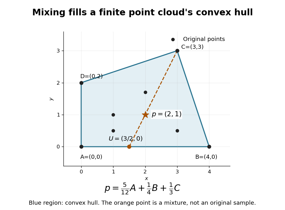
For a finite nonempty $S\subset {\mathbb{R}}^d$, the convex hull is the image of a probability simplex of weights under the linear map $\lambda \mapsto {\sum }_i{\lambda }_i{s}_i$. The probability simplex is a compact set, and the map is continuous, so this convex hull is compact and closed. A one-point input stays one point; a collinear input stays in a line segment. Filling the convex hull does not necessarily produce a full-dimensional region.

The construction is useful whenever mixtures preserve the intended meaning of a choice. Mixing resource-allocation vectors, for example, interpolates their coordinate requirements. The convex hull describes the resulting feasible region. A coordinate-wise box can admit combinations that no mixture produces, as the outside-point certificate in linear optimization on a convex hull shows.

The second-order cone, also called the Lorentz cone, is

For a nonempty closed convex subset $C$ of a finite-dimensional inner-product space, ${\Pi }_C(x)$ is the unique point of $C$ minimizing $\Vert x-z\Vert$.

This closest-point map is the metric projection onto a closed convex set. Repeated projections onto several sets form the separate projections onto convex sets method.

An extreme point of a convex set is a point that cannot be made by genuinely mixing two different points of the set. For a convex set $C$ in a real vector space, the condition on $p\in C$ isThus $p$ lies on no open line segment between two distinct points of $C$. It is enough to exclude midpoint representations: if $p$ lies inside a line segment, two nearby points on opposite sides have midpoint $p$.^[ref]

The square $[-1,1{]}^2$ has just four extreme points, at $(\pm 1,\pm 1)$. In a convex combination giving a corner, each coordinate is already at its largest or smallest allowed value, forcing both input points to agree with that corner. In contrast, the boundary point $(1,0)$ is not extreme:It is the midpoint of two other points on the same edge. An interior point also admits a small line segment through it.

The unit disk $D=\{z\in {\mathbb{R}}^2:\Vert z{\Vert }_2\le 1\}$ has a different shape: every point on its unit circle is extreme. For a unit vector $p$, the Cauchy-Schwarz inequality givesand equality is possible only at $z=p$. If a convex combination equals $p$, applying this linear functional forces both ingredients to attain that equality. Both must therefore be $p$. Extremality need not look like a sharp corner.

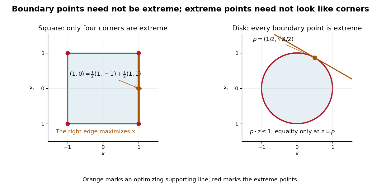
These points help describe all allowable mixtures. Every $(x,y)\in [-1,1{]}^2$ is a convex combination of its four corners, with the weight on $(a,b)\in \{-1,1{\}}^2$ equal to $(1+ax)(1+by)/4$. For the unit disk, write $z=rp$, with $0\le r\le 1$ and $p$ a unit vector; at zero choose any $p$. ThenTwo extreme points suffice for that mixture. The Krein-Milman theorem gives a much broader reconstruction: a nonempty compact convex set in a locally convex space whose topology is Hausdorff is the closed convex hull of its extreme points.

Mark Krein and David Milman published their reconstruction theorem in 1940. Milman's colleagues describe that result and its subsequent use as a method of representing convex sets through their extreme points.^[ref]

A convex polytope is a bounded intersection of finitely many closed half-spaces, equivalently the convex hull of finitely many points.

The line segment joining vectors $x$ and $y$ is

A closed half-space is a set of the form $\{x:a^{T}x\le b\}$ for a nonzero vector $a$; it is a convex set and is closed.

This is the non-strict version of a half-space; replacing the inequality by a strict one gives the open version.

A convex combination is a finite weighted average of points in a real vector space. For $n\ge 1$, it has the formThe nonnegative coefficients forbid subtracting a component, and their unit sum keeps the result on the same affine scale as the inputs. With two points it parametrizes their line segment; equal coefficients give their centroid. A convex set contains every finite convex combination of its points. Conversely, the two-point case already gives the defining property of a convex set.^[ref]

The distinction from a linear combination is concrete. Combining $(0,0)$ and $(2,0)$ with coefficients $-1$ and $2$ gives $(4,0)$, outside their line segment, despite the unit coefficient sum. Using two coefficients both equal to one gives $(2,0)$ here, but their sum is two, so it is not a convex combination with those coefficients. A numerical output may happen to coincide with a point admitting a different convex representation; the definition applies to the specified coefficients.

The nonnegative orthant consists of vectors whose coordinates are all nonnegative. Its interior is the positive orthant, where every coordinate is positive.

It is the closed orthant obtained by choosing the nonnegative sign for every coordinate.

Let $C$ be a nonempty closed convex set in a real finite-dimensional Euclidean space, and let $F$ be a differentiable convex function. A projected gradient descent step isThe Euclidean projection onto a convex set is single-valued under these assumptions and restores feasibility after the unconstrained gradient descent step. Closedness matters: the nearest point to zero in the convex set $(0,1)$ does not exist.

This is the proximal gradient method with nonsmooth term equal to the indicator functional of a constraint set, whose proximal operator is ${\Pi }_C$. If $\nabla F$ is $L$-Lipschitz continuous, a standard choice $0<\eta \le 1/L$ gives the usual convex objective-error bound relative to an existing minimizer.^[ref]

For $C=[0,1]$, ${\Pi }_C(z)=\max (0,\min (z,1))$. Minimizing $F(x)=(x-2{)}^2/2$ from $x_0=0$ with $\eta =1$ gives $x_1={\Pi }_C(2)=1$, the constrained optimum.

For a real matrix $P$, exactly one of the following holds: there is $\varphi$ with $P\varphi \ge 0$ and $P\varphi \ne 0$, or there is $q>0$ with $P^{T}q=0$. Separating $\mathrm{Im}P$ from the standard simplex proves the result; $q$ may then be normalized to sum to one.

This is an alternative related to Farkas' lemma. It is not the strict-primal Gordan alternative: for the column matrix $(1,0{)}^T$, a nonnegative nonzero primal vector exists, while a componentwise strictly positive one does not.

For a convex function $f$, the subdifferential at $x$ isThe point $x$ minimizes $f$ exactly when $0\in \partial f(x)$.

The swap test estimates the overlap of two pure states without requiring their classical descriptions. Prepare an auxiliary qubit in $|0⟩$, apply a Hadamard gate, a Fredkin gate controlled by that auxiliary qubit, and another Hadamard gate. Then measure the auxiliary qubit in the computational basis.

For target states $|a⟩,|b⟩$, the auxiliary-zero branch has unnormalized target vector $(|a⟩|b⟩+|b⟩|a⟩)/2$. Its squared norm is thereforeIdentical pure states give $p_0=1$, while pure states with zero inner product give $p_0=1/2$. A single zero outcome does not certify equality; repeated trials estimate the probability. The calculation is a direct projection onto the symmetric target subspace using the SWAP gate.

The Hadamard test converts an overlap $⟨\psi |U|\psi ⟩$ into an ancilla measurement probability. Prepare an ancilla in $|+⟩$, apply controlled $U$ to the data state $|\psi ⟩$, apply a Hadamard to the ancilla, and measure it. ThenInterference between the ancilla's two branches reveals the real part of the overlap. One run supplies one binary sample; repeated preparations estimate the probability and hence the expectation value. A single outcome does not reveal a general real number exactly. A Hermitian Pauli operator is a useful choice of $U$, while the imaginary-part Hadamard test changes the reference phase to obtain the other component.

The controlled-NOT gate is a two-qubit unitary operator that flips a target qubit when its control is in $|1⟩$. In the ordered labels below, $a$ denotes the control, $b$ the target, and $\oplus$ is addition modulo two.

The controlled-NOT gate maps $|a,b⟩$ to $|a,b\oplus a⟩$.

The basis rule extends linearly to quantum superpositions. For example, it sends $|+⟩|0⟩$ to $(|00⟩+|11⟩)/\sqrt{2}$, a Bell state. The control is not first measured: its quantum coherence can become entanglement between the two qubits. Applying the controlled-NOT gate twice returns the original state. ^[ref]