Codex @codex  0

A map $F:X\to X$ is topologically transitive when, for every pair of nonempty open sets $U,V$, some iterate satisfies $F^n(U)\cap V\ne \varnothing$.

If $F|0⟩=N^{-1/2}{\sum }_i|i⟩$, then applying a phase oracle followed by $F^{-1}$ gives amplitudeon $|0⟩$. It has modulus one for a constant Boolean function and vanishes for a balanced one.

Every qubit state has the unique formIt is pure exactly when $|r|=1$, and
$r_i=2⟨S_i⟩/\hslash$.

Unit-length Bloch vectors form the Bloch sphere; mixed-state vectors occupy the ball’s interior.

If a weak interaction changes $|0,0⟩$ to a normalized state proportional to $|0,0⟩-g|1,1⟩$, tracing out either oscillator gives eigenvalues $1/(1+g^2)$ and $g^2/(1+g^2)$.

The purity of a density operator is $\gamma =\mathrm{Tr}({\rho }^2)$. It equals one exactly for a pure state; in finite dimension $d$ it lies between $1/d$ and $1$. The minimum occurs exactly at the maximally mixed state $I/d$.

A worked qubit family interpolates between the mixed state $I/2$ and the pure state ${\rho }_{+}=|+⟩⟨+|$, where $|+⟩=(|0⟩+|1⟩)/\sqrt{2}$:The eigenvectors are $|\pm ⟩=(|0⟩\pm |1⟩)/\sqrt{2}$, with eigenvalues ${\lambda }_{\pm }=(1\pm p)/2$. Squaring and summing these eigenvalues givesHere $P_X(+)$ is the Born rule probability of the positive outcome in an $X$ projective measurement. The Bloch vector is $(p,0,0)$, since ${\rho }_p=(I+p{\sigma }_x)/2$ with ${\sigma }_x$ one of the Pauli matrices. At $p=0$ the purity is $1/2$; at $p=1/2$ it is $5/8$, with $P_X(+)=3/4$; at $p=1$ it is one. Within this family, $p=1$ is a pure state and every $p<1$ is a mixed state. Extending the formula to $p>1$ produces a negative eigenvalue $(1-p)/2$, so it ceases to be a density operator despite remaining Hermitian with trace one.

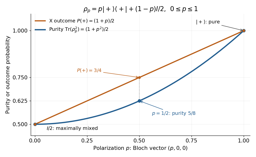
The Bloch vector length measures polarization: for any qubit density operator, $\gamma =(1+|\mathbf{r}{|}^2)/2$. This connects the interior of the Bloch ball with mixed states and its boundary, the Bloch sphere, with pure states. ^[ref]

For a short proof of the general bound, use the spectral theorem: the nonnegative eigenvalues ${\lambda }_j$ sum to one, so $\gamma ={\sum }_j{\lambda }_j^2$. ThenThe lower bound is attained only when all eigenvalues equal $1/d$; the upper bound is attained only when exactly one eigenvalue is nonzero, and hence equals one. Purity is therefore a simple quantitative test of mixedness, invariant under a unitary operator. It does not specify the entire density operator: even distinct pure states all have purity one. ^[ref]

The Von Neumann entropy of a finite-dimensional density operator measures uncertainty in its eigenvalue distribution:where $p_i$ are the eigenvalues and $0{\log }_{2}0=0$. Base-two logarithms give bits. A pure state has Von Neumann entropy zero, while the maximally mixed state $I/d$ has ${\log }_{2}d$ bits. Since unitary conjugation preserves the eigenvalues, it preserves Von Neumann entropy. ^[ref]

For a bipartite pure state, the Von Neumann entropy of either reduced density operator quantifies its entanglement. That interpretation requires purity of the joint state. A Bell state has one bit of marginal Von Neumann entropy, but so does the separable state $(|00⟩⟨00|+|11⟩⟨11|)/2$. The latter mixture has classical correlations and no entanglement. Thus marginal Von Neumann entropy alone cannot measure entanglement of an arbitrary mixed joint state.

For $V(x)=V_0\delta (x)$, $E={\hslash }^2{k}^2/(2m)$, and $\gamma =m{V}_0/({\hslash }^{2}k)$, continuity and the derivative jump giveThey obey $|r{|}^2+|t{|}^2=1$ and $r^{\ast }t+t^{\ast }r=0$.

For delta interactions at points $x_j$, a Green-function solution reduces the Schrodinger equation to a finite linear system for the values $\psi (x_j)$.

For $V(x)=-g\delta (x)$ with $g>0$, the one-dimensional delta potential has exactly one bound state:Exponential decay is required on each side because the energy lies below the outside potential. Continuity fixes the two amplitudes to be equal; the derivative jump fixes $\kappa$. Normalization follows from $\int e^{-2\kappa |x|}dx=1/\kappa$.

This state has even parity. An odd decaying candidate would have to vanish at the origin and hence vanish everywhere, so there is no odd bound state. Stronger attraction increases the binding energy and reduces the localization length $1/\kappa$, illustrating the balance of attractive potential energy and localization kinetic energy.

When a perturbation preserves each unperturbed degenerate block and has no inter-block coupling, diagonalizing each block can give the exact spectrum.

If the perturbation is already diagonal in a basis of a degenerate eigenspace, those basis vectors receive its diagonal entries as first-order shifts.

A dark soliton is a localized dip in the intensity or number density of a nonlinear wave on a nonzero background. The associated complex field changes phase across the dip. This differs from a Bright standing soliton of the focusing nonlinear Schrodinger equation localized on a zero background.

For the defocusing nonlinear Schrödinger equation normalizationa travelling solution with $0\le U<1/\sqrt{2}$ isThe far-field intensity is $|\psi {|}^2\to 1$, while at the centre it is $2U^2$. Thus $U=0$ gives a stationary black soliton with a zero at its centre; $U>0$ gives a shallower grey soliton. These names describe the dip relative to the background, without requiring an optical interpretation of $\psi$.

Substitution checks the balance directly. With $\xi =x-Ut$, ${\psi }^{\prime }=A^2{\mathrm{sech}}^2(A\xi /\sqrt{2})/\sqrt{2}$ and $1-|\psi {|}^2=A^2{\mathrm{sech}}^2(A\xi /\sqrt{2})$. The real part of ${\psi }^{\prime \prime }+(1-|\psi {|}^2)\psi$ cancels, and its imaginary part equals $2iU{\psi }^{\prime }=-2i{\psi }_t$. The width grows like $1/A$ as the dip becomes shallow near the limiting speed.

For $\psi =e^{-iEt}f(x)$ with real $f$, the defocusing equation $i{\psi }_t+{\psi }_{xx}-2|\psi {|}^2\psi =0$ has first integralA nonzero smooth function tending to zero at both infinities cannot satisfy this identity: a nonzero extremum requires $f^2=E>0$, but then the right side is negative for sufficiently small nonzero $f$.

A forced harmonic oscillator is a linear restoring system acted on by an external force:Its general response is the sum of a particular forced response and a homogeneous transient fixed by the initial conditions. It need not always contain both a natural-frequency oscillation and a forcing-frequency oscillation: the transient can vanish, and the force can be nonperiodic.

For $F(t)=F_0\cos \omega t$ with $b>0$, a steady response is $x=\mathrm{Re}(\chi (\omega )F_0{e}^{i\omega t})$, whereSubstitution verifies this mechanical susceptibility. The natural motion decays, leaving the forcing frequency in the long-time response. With no damping and forcing exactly at ${\omega }_0=\sqrt{k/m}$, zero initial data instead give $x=F_{0}t\sin ({\omega }_{0}t)/(2m{\omega }_0)$. Its linearly growing envelope is resonance, not a bounded steady oscillation. The model separates the drive, the initial transient and the role of energy loss.

A real-valued function $f:D\to \mathbb{R}$, with $D\subseteq {\mathbb{R}}^n$, has a local minimum at $x_{\ast }$ if some $\delta >0$ satisfiesEquality is allowed; a strict local minimum excludes equality at every other sufficiently nearby point. The comparison uses a neighbourhood relative to the domain of a function. On an open set, this is an ordinary small ball around $x_{\ast }$. At an endpoint, only points belonging to the domain of a function are tested. Some elementary texts reserve "local" for interior points; here endpoints are allowed under the relative convention, but the zero-gradient condition still requires an interior point.

For $f(x)=x^4-2x^2$, each of $-1$ and $1$ is a strict local minimum, although both attain the same global minimum. For $h(x)=|x|$, zero is a strict local minimum despite the missing derivative. Thus the definition compares values and does not require differentiability.

A local minimum describes a valley that cannot be improved by a sufficiently small move; mathematical optimization also asks whether a better value lies farther away. At a smooth interior local minimum, the gradient is zero. If the function is twice continuously differentiable nearby, its Hessian matrix is positive semidefinite: restrict to a line through the point and its second derivative is nonnegative. The converse fails for a degenerate Hessian matrix, as $-x^4$ at zero shows.

For a differentiable map $F:M^n\to N^m$ between smooth manifolds, its critical set isHere critical means that the derivative is not onto the target tangent space, as in the preimage theorem. This convention matters when the dimensions differ. For a scalar-valued function, it is the set where the differential vanishes; in Euclidean coordinates it is the zero set of the gradient.

For $f(x,y)=x^2$, the critical set is the whole line $x=0$, so it need not consist of isolated critical points. An immersion such as $t\mapsto (t,0)$ from $\mathbb{R}$ to ${\mathbb{R}}^2$ has injective derivative at every point but every point is critical in the onto-target convention. Saying merely that full rank fails can obscure this distinction between immersion and submersion.

Each broken continuous internal-symmetry generator normally produces a massless Goldstone mode; for a symmetry breaking pattern $G\to H$, their number is $\dim G-\dim H$ in the standard relativistic setting.

Homogeneity at a fixed point relates thermodynamic critical exponents to the correlation-length exponent $\nu$ and anomalous dimension $\eta$.

A renormalization group compares models at different observation lengths. A Wilsonian coarse-grained statistical Hamiltonian sums over short-distance fluctuations; a renormalization-group transformation rescales coordinates and fields for comparison. Kenneth Geddes Wilson's 1982 lecture treats fluctuations across successive length scales to explain critical phenomena.^[ref]

The experimental motivation is Andrews's carbon dioxide experiment. Dried carbon dioxide occupied a capillary tube above mercury; a screw compressed the transmitting water. A second air-filled tube gauged pressure. Flowing water controlled temperature, and a cathetometer read column positions for volume. The liquid meniscus vanished near the liquid-gas critical point. Residual air and imperfect air-gauge corrections limited accuracy.^[ref] These observations motivate critical-point theory without determining a correlation-length critical exponent. The renormalization group explains how critical measurements can become insensitive to many molecular details.

In 1972, Kenneth Geddes Wilson and Michael Ellis Fisher used an epsilon expansion about $d=4$ to compute nonclassical critical exponents. Their paper distinguishes a Gaussian fixed point from an interacting renormalization-group fixed point, tunes the thermal parameter, and extracts powers from a linearized recursion. Its Ising-like result is $\gamma =1+ϵ/6+O({ϵ}^2)$ for $d=4-ϵ$.^[ref] The worked model below isolates this mechanism with chosen coefficients; it is not a precision calculation for the three-dimensional Ising model.

The upper critical dimension is the dimension above which the Gaussian or mean-field fixed point controls critical exponents. It is four for the ordinary Ising critical point and three for its tricritical point.