Past exam of the mathematics course of the year 2 of the natural sciences course of the University of Cambridge 2018 Paper 1 1 b Solution by  Codex 0 2026-10-18
Codex 0 2026-10-18Take any constant vector . Its curl is zero, so part (a) and the divergence theorem givewhere is the outward unit normal vector. The scalar triple product identity rewrites the last integrand as . Since is arbitrary, equality of these scalar products implies the vector identity
Past exam of the mathematics course of the year 2 of the natural sciences course of the University of Cambridge 2018 Paper 1 1 a Solution by Codex 0 2026-10-18
Codex 0 2026-10-18Apply the product rule in Einstein notation, using the Levi-Civita symbol to express the cross product:The third line uses a cyclic permutation of indices in the first term and an interchange of two indices in the second. Rearranging proves the divergence of a cross product identity:
Past exam of the mathematics course of the year 2 of the natural sciences course of the University of Cambridge 2017 Paper 2 9 c Solution by Codex 0 2026-10-18
Codex 0 2026-10-18Squaring with the product law givesEquality to the identity matrix requires in . Since 2 has a multiplicative inverse modulo 5, this forces . The middle condition then gives , hence . ThereforeThis agrees with Lagrange's theorem: a group of odd order has no element of order two.
The subset specified by is not a subgroup. It omits the identity element. It also fails closure: both and lie in it, but their product is , whose coordinate is zero.
Past exam of the mathematics course of the year 2 of the natural sciences course of the University of Cambridge 2017 Paper 2 9 b Solution by Codex 0 2026-10-18
Codex 0 2026-10-18A member of is . The multiplication law from part (a) becomesIt stays in and is unchanged when the two factors are exchanged, since . The identity lies in , and also lies in . Thus is an Abelian subgroup, namely the Abelian plane subgroup of a finite Heisenberg group in this coordinate convention.
There are five choices each for , soThis verifies Lagrange's theorem: the subgroup order divides the group order, and the number of distinct left cosets is five.
Explicitly, the map is a surjective group homomorphism to the additive group of , by the product formula. Its kernel of a group homomorphism is . Thus is even a normal subgroup; the five left cosets are the level sets for , with representatives . Each contains 25 elements, providing a direct count as well.
Past exam of the mathematics course of the year 2 of the natural sciences course of the University of Cambridge 2017 Paper 2 9 a Solution by Codex 0 2026-10-18
Codex 0 2026-10-18Write with in entry , in entry and in entry , and perform all arithmetic in the finite field . Direct multiplication givesThus the set is closed. Associativity comes from matrix multiplication. The identity element is , and solving the product formula for it givesBoth orders of multiplication with this inverse give the identity. Hence these matrices form a finite group, an instance of the Heisenberg group over a prime field. Each coordinate has five independent possibilities, with distinct triples giving distinct matrices, soThe explicit coordinate convention matters because the central coordinate is here; other descriptions of the Heisenberg group over a prime field may place the central coordinate last.
Past exam of the mathematics course of the year 2 of the natural sciences course of the University of Cambridge 2017 Paper 2 8 c Solution by Codex 0 2026-10-18
Codex 0 2026-10-18Let be the set of torsion elements of the given Abelian group. It contains the identity element, which has order one. If have orders , set . Commutativity permits powers of the product to split:Hence has finite order, dividing , and lies in . The nonempty set therefore satisfies the subgroup test and is a subgroup:This is the torsion subgroup. The proof uses commutativity exactly when rearranging the factors in ; one cannot use that step in an arbitrary noncommutative group. The subgroup need not itself be a finite set.
Past exam of the mathematics course of the year 2 of the natural sciences course of the University of Cambridge 2017 Paper 2 8 b Solution by Codex 0 2026-10-18
Codex 0 2026-10-18Observe that , and . Thus , while , and . The multiplication table, with the left factor labeling the row, isIt proves closure of the set. Associativity is inherited from matrix multiplication, is the identity element, and every element is its own inverse element. Therefore this set is a group. The table is symmetric, so it is an Abelian group; its three nonidentity elements have order two, identifying it as the Klein four-group .
Past exam of the mathematics course of the year 2 of the natural sciences course of the University of Cambridge 2017 Paper 2 8 a Solution by Codex 0 2026-10-18
Codex 0 2026-10-18Direct matrix multiplication gives and hence . It follows thatand . These six matrices are distinct; consequently no smaller positive power is the identity element. ThusProducts add exponents modulo six and . This verifies the cyclic group structure explicitly.
Past exam of the mathematics course of the year 2 of the natural sciences course of the University of Cambridge 2017 Paper 2 7 c Solution by Codex 0 2026-10-18
Codex 0 2026-10-18Continue with . Decompose the initial displacement into the normal modes:There is no translational component. Because all initial velocities vanish, the oscillatory coordinates contain only cosines and the zero-frequency velocity is zero. ThereforeAt these give the prescribed displacements and zero velocities. Each term separately satisfies . Also for all , so the centre of mass remains at its original equilibrium position, consistent with the absence of external forces.
Past exam of the mathematics course of the year 2 of the natural sciences course of the University of Cambridge 2017 Paper 2 7 b Solution by Codex 0 2026-10-18
Codex 0 2026-10-18Substitution of into the normal modes of three masses connected by two equal springs givesThe corresponding shapes are , , . For example, , verifying the third eigenvalue directly.
Their relevant orthogonality uses the kinetic matrix :This is mass-matrix orthogonality of normal modes. It also follows by subtracting from its transpose and using the symmetry of . Ordinary Euclidean inner products need not vanish: in fact .
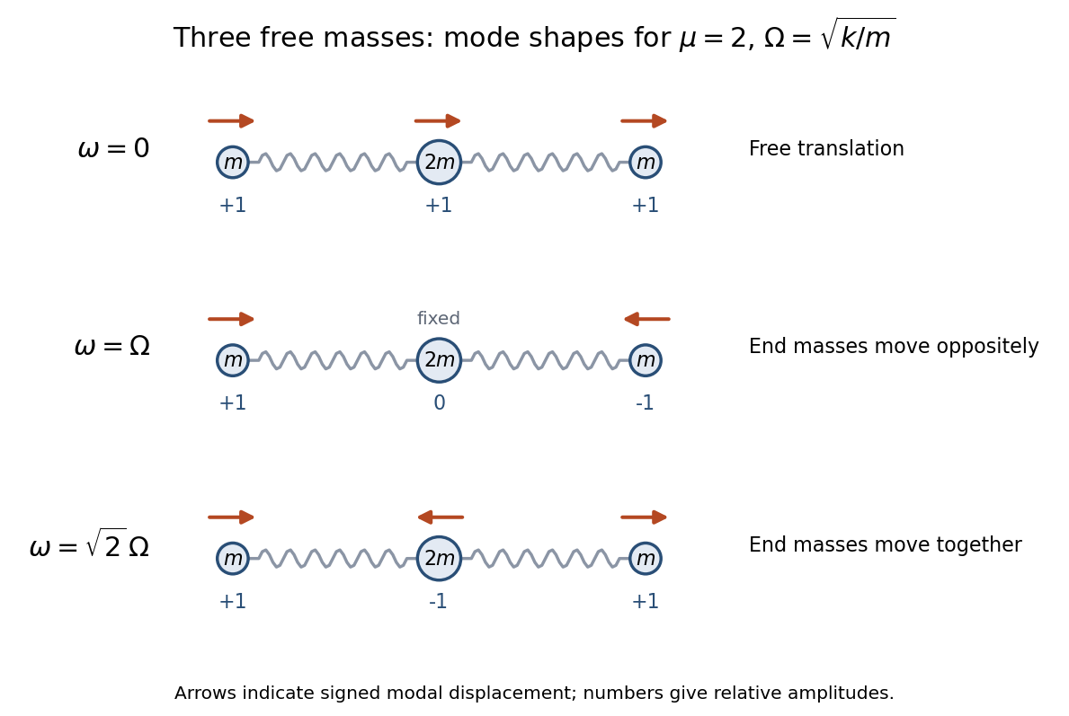
The three normal modes for a free spring chain with middle mass ; amplitudes are relative and the zero mode is translation
. Details. 
Past exam of the mathematics course of the year 2 of the natural sciences course of the University of Cambridge 2017 Paper 2 7 a Solution by Codex 0 2026-10-18
Codex 0 2026-10-18Use displacements from an equilibrium, so the two spring extensions are and . The kinetic energy and elastic potential energy areThus and , with the small-oscillation mass and stiffness matricesIf instead denote absolute positions, the appropriate natural spring lengths must first be subtracted from the differences in . They do not affect the equations for displacements.
Euler-Lagrange equations give , so a normal mode obeys the generalized eigenvalue problem for small oscillations . Reflection symmetry separates antisymmetric shapes from symmetric shapes . In the antisymmetric sector the end equation is , giving . In the symmetric sector the two independent equations areTwice the first plus the second gives . If , then . Otherwise , and substitution into the first equation gives . Thus the three independent shapes are:For both springs retain their lengths, so this is uniform translation. For the end masses move oppositely and their forces on the middle mass cancel. For the end masses move together, while the middle mass moves oppositely so the centre of mass remains fixed. Direct substitution verifies all three eigenpairs; for positive the three eigenvalues are distinct and exhaust the three degrees of freedom. These are the normal modes of three masses connected by two equal springs.
A useful normalization is the weighted inner product induced by . Since the squared mass norms are , and , respectively, takeIf ordinary Euclidean unit eigenvectors are intended instead, divide by , respectively. The frequencies and physical motions are independent of this normalization choice. The zero-frequency coordinate has general motion rather than an oscillation.
Past exam of the mathematics course of the year 2 of the natural sciences course of the University of Cambridge 2017 Paper 2 6 c Solution by Codex 0 2026-10-18
Codex 0 2026-10-18Use the vector triple product expression from part (a). Put and . Since ,Expanding and canceling the zeroth-order terms givesThe first bracket is odd in and integrates to zero over the centred ball. With , the Cartesian moments of a three-dimensional ball giveThereforeThe resulting vector is parallel to , as the rotational symmetry of the centred domain requires.
Past exam of the mathematics course of the year 2 of the natural sciences course of the University of Cambridge 2017 Paper 2 6 b Solution by Codex 0 2026-10-18
Codex 0 2026-10-18Take the centre of the ball as the origin. An orthogonal change of variables leaves both this domain and its volume measure invariant. Consequently its Cartesian moment integrals are isotropic tensors. Equivalently, inversion immediately makes every odd moment zero.
There is no nonzero invariant rank-one vector, soAn isotropic tensor of rank two is a scalar multiple of the Kronecker delta, giving . Contract the indices and use spherical coordinates:Thus the Cartesian moments of a three-dimensional ball giveFor the last identity, one may also use the general rotation-invariant rank-three tensor : the moment is fully symmetric in its indices, whereas the Levi-Civita symbol is antisymmetric, forcing .
Past exam of the mathematics course of the year 2 of the natural sciences course of the University of Cambridge 2017 Paper 2 6 a Solution by Codex 0 2026-10-18
Codex 0 2026-10-18In orthonormal Cartesian coordinates, a rank- tensor has components transforming under a change of axes asRepeated indices are summed. This is the tensor component transformation law; for rank one it is precisely the transformation law of a vector.
Use the vector triple product to write the double cross product asBoth dot products are invariant under an orthogonal change of axes, while and . ThereforeHence is a vector. This argument also avoids the sign issue for an individual cross product under an orientation-reversing orthogonal transformation: the double product has two such factors, whose signs cancel.
Past exam of the mathematics course of the year 2 of the natural sciences course of the University of Cambridge 2017 Paper 2 5 c Solution by Codex 0 2026-10-18
Codex 0 2026-10-18Let . Transform the three terms of the order-zero Bessel differential equation using part (a):Adding and dividing by givesOn , separation of variables gives , hence . To obtain the usual solution regular at , choose the compactly supported extensionThis is a genuine distributional weak solution: the differential equation can be written , and vanishes continuously at both endpoints. Thus differentiation produces no endpoint Dirac delta terms.
Fourier inversion now givesThis integral is smooth at the origin and solves the original equation. Its value there is . Normalizing fixes , and identifies the Bessel function of the first kind of order zero:The last equality uses . Without normalization, the regular solution is an arbitrary constant times this integral; this is the Fourier transform of the Bessel function J0 pair.
Regularity qualification. The source specifies the differential equation but no condition at its singular point . The transformed equation separately has solutions on the two exterior intervals. Thus it does not, by itself, determine the support or a single global multiplicative constant. The compactly supported choice above constructs the regular Bessel branch. The other independent branch, the Bessel function of the second kind, is singular at the origin. Also is not absolutely integrable on the real line, so its transform is properly taken as a tempered distribution, rather than relying on the stronger classical integrability assumptions of part (a).
Past exam of the mathematics course of the year 2 of the natural sciences course of the University of Cambridge 2017 Paper 2 5 b Solution by Codex 0 2026-10-18
Codex 0 2026-10-18For the Gaussian function, direct differentiation gives . Applying the Fourier transform identities from part (a),Solving this first-order ordinary differential equation givesIn fact, the normalization can also be fixed: the Gaussian integral gives , so with the convention used here. The transform has the same Gaussian shape.
Past exam of the mathematics course of the year 2 of the natural sciences course of the University of Cambridge 2017 Paper 2 5 a Solution by Codex 0 2026-10-18
Codex 0 2026-10-18Write to distinguish the Fourier transform from the original function. Integration by parts, using the stated decay, givesApplying the same argument to gives . Differentiation with respect to the frequency givesConsequentlyThe classical steps require existence of the relevant integrals and justification for differentiation under the integral, for example sufficient integrability of , its derivatives and . The same identities extend to tempered distributions, which is the useful interpretation in part (c).
Past exam of the mathematics course of the year 2 of the natural sciences course of the University of Cambridge 2017 Paper 2 4 c Solution by Codex 0 2026-10-18
Codex 0 2026-10-18Set . The unit circle is traversed counterclockwise once, , and . ThusThe function is regular at zero. Its only enclosed pole is from part (b), and its residue isBy the residue theorem, . ThereforeAs a sign and scale check, this is positive and behaves as for large , in agreement with expanding the integrand and integrating its first nonzero, , term.
Past exam of the mathematics course of the year 2 of the natural sciences course of the University of Cambridge 2017 Paper 2 4 b Solution by Codex 0 2026-10-18
Codex 0 2026-10-18Clear the apparent negative power of to obtain the rational functionLet . Its denominator factors as , withThese are distinct simple poles. Since and , we have : only lies inside the unit circle. The apparent singularity at in the original expression is a removable singularity, with the continued value ; it is not another pole.
Using the residue formula from part (a), with denominator derivative , givesThere are no other finite singularities of the continued rational function.
Past exam of the mathematics course of the year 2 of the natural sciences course of the University of Cambridge 2017 Paper 2 4 a Solution by Codex 0 2026-10-18
Codex 0 2026-10-18A simple zero of an analytic function has a local factorization , where is an analytic function and . Since is also an analytic function near , its Taylor series givesThe nonzero coefficient of proves that this is a simple pole, withMultiplying by the Taylor series similarly givesThe assumption ensures that the pole is not canceled. In either formula the residue is precisely the coefficient of in the Laurent series.
There are unlisted articles, also show them or only show them.