Past exam of the mathematics course of the year 2 of the natural sciences course of the University of Cambridge 2017 Paper 1 1 a Solution by  Codex 0 2026-10-18
For a continuously differentiable vector field on a bounded volume with piecewise smooth closed boundary , the divergence theorem stateswhere is the outward unit normal vector. Thus total outward flux through a closed surface equals the integral of the local divergence inside it. A nonclosed surface first needs a suitable closure, with the added surface's flux accounted for separately.
Past exam of the mathematics course of the year 2 of the natural sciences course of the University of Cambridge 2016 Paper 2 9 c Solution by Codex 0 2026-10-18
Codex 0 2026-10-18Let be a proper subgroup. By Lagrange's theorem, divides . Since , its possibilities areThe subgroup of order one is generated by the identity and is cyclic. For either prime order or , choose other than the identity. Its order of a group element divides and is not one, so it is . Thus its powers exhaust , proving .
ThereforeThis uses the fact that a group of prime order is cyclic. It does not require the order-21 group itself to be Abelian or cyclic.
Past exam of the mathematics course of the year 2 of the natural sciences course of the University of Cambridge 2016 Paper 2 9 b Solution by Codex 0 2026-10-18
Codex 0 2026-10-18A group homomorphism is a map preserving multiplication:It necessarily sends to and sends inverses to inverses, by applying this relation to and . Its kernel of a group homomorphism isThe kernel is a normal subgroup of the domain: if and , then . The kernel’s identity condition refers to the identity in the target group.
Past exam of the mathematics course of the year 2 of the natural sciences course of the University of Cambridge 2016 Paper 2 9 a Solution by Codex 0 2026-10-18
Codex 0 2026-10-18Write with . For any , the normal subgroup property implies . This conjugate cannot be , since multiplication by and would then give . There is only one remaining choice, soThus commutes with every element of ; the identity does too. HenceThis proves that a normal subgroup of order two is central. The proof does not require to be finite: conjugation permutes and fixes its identity, so it must fix its only other element.
Past exam of the mathematics course of the year 2 of the natural sciences course of the University of Cambridge 2016 Paper 2 8 c Solution by Codex 0 2026-10-18
Codex 0 2026-10-18For every positive integer , the group laws give . ConsequentlyThe sets of positive exponents returning the two elements to the identity element are identical. If this set is nonempty, its least member is the order of a group element in both cases. If it is empty, neither element has finite order. Therefore, including the infinite-order case,For a direct divisibility argument in the finite case, if has order , then , so its inverse’s order divides . Reversing the roles shows divides that order, forcing equality. This is the general fact that an element and its inverse have the same order; it also reflects as cyclic subgroups.
Past exam of the mathematics course of the year 2 of the natural sciences course of the University of Cambridge 2016 Paper 2 8 b Solution by Codex 0 2026-10-18
Codex 0 2026-10-18The four displayed matrices fail closure: for example is not one of them. Thus they do not form a group by themselves.
Let and . The enlarged set is the single-qubit Pauli groupThere are 16 distinct matrices: are linearly independent, so two different ones cannot be scalar multiples, and the four phases are distinct for each nonzero matrix.
The Pauli matrices satisfyHere is the Kronecker delta and the Levi-Civita symbol. Thus any product of two Pauli matrices is another Pauli matrix or the identity times a phase in . Multiplying by the two original phases preserves membership in , proving closure of all 16 matrices.
Associativity is inherited from matrix multiplication, the identity is , andThis proves every group axiom. The resulting group is non-Abelian, since reversing changes its sign.
Past exam of the mathematics course of the year 2 of the natural sciences course of the University of Cambridge 2016 Paper 2 8 a Solution by Codex 0 2026-10-18
Codex 0 2026-10-18The quotient group consists of the cosets , with multiplicationFor well-definedness, replacing representatives by and changes their product to . Since is a normal subgroup, the final two factors lie in , so the product coset does not change.
Associativity follows from that in ; the identity element is the coset , and . Hence these cosets form a group. By Lagrange's theorem, every subgroup has order dividing , and its subgroup index is . In particularNormality is needed for the quotient multiplication, whereas Lagrange’s counting formula holds for every subgroup.
Past exam of the mathematics course of the year 2 of the natural sciences course of the University of Cambridge 2016 Paper 2 7 c Solution by Codex 0 2026-10-18
Codex 0 2026-10-18Keep the constraint from part (b). For equal masses and spring constants, the generalized eigenvalue problem for small oscillations reduces toThe horizontal coordinate decouples, givingIn this normal mode, mass 1 oscillates horizontally, mass 2 has its horizontal coordinate fixed, and neither mass has a vertical displacement.
For the vertical block, write . Its characteristic polynomial is . Thus , and the first vertical equation gives . If is the golden ratio, the two vertical modes areIn the lower-frequency mode, the masses move vertically in phase, with the lower mass having the larger amplitude. In the higher-frequency mode they move oppositely, with lower-to-upper amplitude ratio . Their Euclidean inner product is zero because ; since , this is also mass-matrix orthogonality of normal modes.
The three frequencies satisfy . Each mode has a scalar coordinate , and their superposition gives the general constrained motion. No zero-frequency mode remains because the first spring anchors the system. Gravity fixes the equilibrium extensions but drops out of these frequencies for zero-natural-length springs.
Past exam of the mathematics course of the year 2 of the natural sciences course of the University of Cambridge 2016 Paper 2 7 b Solution by Codex 0 2026-10-18
Codex 0 2026-10-18At equilibrium, the two horizontal equations imply and then , so both vanish. Adding the two vertical equations gives ; the second separately gives . HenceRetain the imposed constraint and set , , . Subtracting the equilibrium equations cancels all constant gravitational terms. For , the small-oscillation mass and stiffness matrices areThe horizontal reaction enforcing the constraint replaces the removed equation; it is not necessary to demand that the original unconstrained horizontal force on mass 2 vanish during motion. Because the zero-natural-length spring potentials are exactly quadratic, these displacement equations are actually exact within the ideal spring model, not merely first-order approximations.
Past exam of the mathematics course of the year 2 of the natural sciences course of the University of Cambridge 2016 Paper 2 7 a Solution by Codex 0 2026-10-18
Codex 0 2026-10-18For a zero-natural-length spring, extension is the full distance between its endpoints, so the squared spring lengths are quadratic functions of the Cartesian coordinates. The Lagrangian isThe gravitational potential energy has positive derivative in the upward coordinate, giving downward forces. Applying the Euler-Lagrange equations to all four coordinates givesThe two spring forces are equal and opposite on the two masses for the connecting spring, as required by Newton's third law.
Past exam of the mathematics course of the year 2 of the natural sciences course of the University of Cambridge 2016 Paper 2 6 d Solution by Codex 0 2026-10-18
Codex 0 2026-10-18For , the inertia tensor component is . Reflect either coordinate appearing once: the cylindrical domain and density are unchanged, while the integrand changes sign. Thus every off-diagonal component vanishes. Rotational symmetry also implies .
Use cylindrical coordinates , , , with volume element . The axial moment of inertia isThe two contributions to a transverse component areThereforeThe axial value and transverse value for , give an independent check on both diagonal entries.
Past exam of the mathematics course of the year 2 of the natural sciences course of the University of Cambridge 2016 Paper 2 6 c Solution by Codex 0 2026-10-18
Codex 0 2026-10-18Use the quarter-turn rotation matrixFor a general second-order tensor, direct multiplication givesRequiring gives , , together with , and together with . Thus all mixed axial-transverse entries vanish andFor an arbitrary rotation angle , the transverse rotation is , where . The transverse block of is , so it commutes with . Therefore , while the axial component is unchanged.
Hence invariance holds under every rotation about the axis, not just the quarter-turn. This is the general axisymmetric second-order tensor; a symmetric tensor would additionally require , but that restriction was not assumed.
Past exam of the mathematics course of the year 2 of the natural sciences course of the University of Cambridge 2016 Paper 2 6 b Solution by Codex 0 2026-10-18
Codex 0 2026-10-18Let be an orthogonal change of axes. Since is a second-order tensor, . The scalar-contraction assumption givesfor every tensor . In one fixed frame its components can be any array: in particular, choose one component at a time to be one, all others zero. Equality of the coefficients then forcesMultiplying by and yieldsThis is exactly the tensor component transformation law. It is the full-contraction version of the quotient theorem for Cartesian tensors. The words “for every” are essential: testing a single , such as the zero tensor or the identity, would not determine all components.
Past exam of the mathematics course of the year 2 of the natural sciences course of the University of Cambridge 2016 Paper 2 6 a Solution by Codex 0 2026-10-18
Codex 0 2026-10-18A second-order Cartesian tensor assigns components in each orthonormal coordinate system according toHere is the matrix taking old vector components to new ones, and repeated indices are summed. This is the tensor component transformation law; an arbitrary array of nine numbers is not a tensor unless its components in different frames obey this rule. No symmetry is implied by being a second-order tensor.
Past exam of the mathematics course of the year 2 of the natural sciences course of the University of Cambridge 2016 Paper 2 5 c Solution by Codex 0 2026-10-18
Codex 0 2026-10-18Factor the cubic denominator as . Substitution givesThere is a double pole at and simple poles at . For , close the inverse-transform contour counterclockwise in the upper half-plane. The residue at the double pole isand the residue at is . Multiplication by from the residue theorem therefore gives .
For , the clockwise lower closure encloses only , with residue . The orientation supplies , giving . Hence the continuous solution isThe large inverse-transform arcs vanish: the rational factor is , while the exponential is bounded on the appropriate closure.
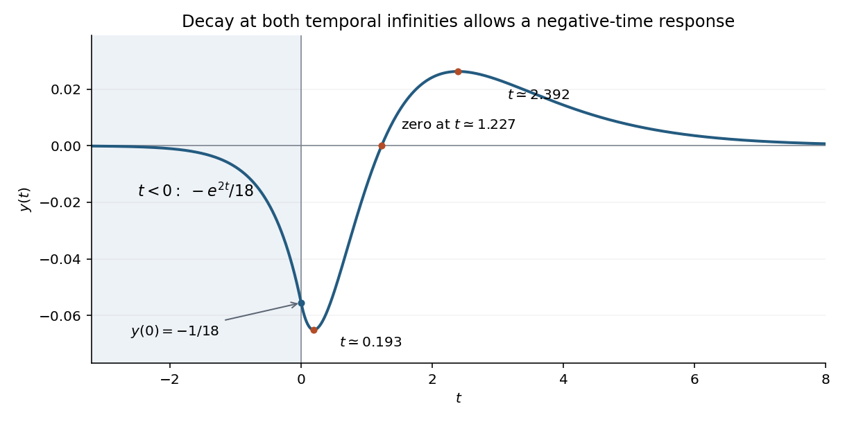
The two-sided decaying Fourier solution; it and its first derivative are continuous at zero
. Details. 
The graph tends to zero from below as , passes through with slope , reaches a small negative minimum after zero, then crosses the axis, reaches a positive maximum and tends to zero from above. The positive-time stationary points solve , and the crossing solves ; these equations determine the sketch without guessing signs.
For a distributional check, and are continuous, while . The jump conditions for a third-order Green function therefore produce the delta in , and each smooth branch satisfies the remaining equation. The nonzero solution for is consistent with the stipulated decay at both temporal infinities. Those are two-sided conditions, not a causality assumption: this is the setting of a decaying two-sided Green function of a constant-coefficient ordinary differential equation and causality versus stability of a Green function.
Past exam of the mathematics course of the year 2 of the natural sciences course of the University of Cambridge 2016 Paper 2 5 b Solution by Codex 0 2026-10-18
Codex 0 2026-10-18The inverse Fourier transform isFor , close in the upper half-plane, where decays. The single enclosed pole has residue , so counterclockwise integration gives . For , close clockwise in the lower half-plane; there is no enclosed pole and the result is zero. ThusHere is the Heaviside step function. At the jump, symmetric Fourier inversion gives , the average of the one-sided limits. The transform itself cannot fix a function’s value at a single point, so this is the conventional representative rather than extra frequency information.
Past exam of the mathematics course of the year 2 of the natural sciences course of the University of Cambridge 2016 Paper 2 5 a Solution by Codex 0 2026-10-18
Codex 0 2026-10-18Take the Fourier transform convention , with inverse factor . Then , classically when the boundary terms vanish or in the sense of tempered distributions.
Multiply the given frequency relation by its denominator and then by :Recognizing the four derivative multipliers givesThe convention is stated explicitly because reversing the Fourier exponential changes intermediate frequency signs. The distributional form will matter at the jump of in part (b).
There are unlisted articles, also show them or only show them.