Past exam of the mathematics course of the year 1 of the natural sciences course of the University of Cambridge 2016 Paper 2 14 c iii Solution by  Codex 0 2026-10-18
From , we have . Substitution into the original relation gives , soThese are real parabola branches, with either sign of allowed when the branch is real. For , differentiating gives and verifies both the relation and the slope. Use graph intervals with and , so the slope is finite and . The separate constant-slope case gives , also represented by the degenerate choice . Squaring has not imposed a sign on , so both real graph branches must be included.
Past exam of the mathematics course of the year 1 of the natural sciences course of the University of Cambridge 2016 Paper 2 14 c ii Solution by Codex 0 2026-10-18
Codex 0 2026-10-18For , separate variables and use partial fraction decomposition:Integration yieldsOn any connected solution interval, absorb the fixed signs into a real constant to writeThe two real signs of the square root are chosen consistently on a branch where . The constant solutions of the reduced equation are . The original equation excludes the last two; is retained by for .
Past exam of the mathematics course of the year 1 of the natural sciences course of the University of Cambridge 2016 Paper 2 14 c i Solution by Codex 0 2026-10-18
Codex 0 2026-10-18Let , so that . Differentiation givesMove the first term to the left and useSince for real and , cancellation givesThis is the slope parameter for a homogeneous first-order equation reduction.
Past exam of the mathematics course of the year 1 of the natural sciences course of the University of Cambridge 2016 Paper 2 14 b ii Solution by Codex 0 2026-10-18
Codex 0 2026-10-18Yes: . Its derivative is , while substitution into the right-hand side gives . This is the equilibrium of the transformed autonomous differential equation; it must be restored separately after dividing by in the separated solution.
It is the only straight-line solution. Substituting into the original equation shows that would require from the coefficients, but the constant coefficients would then give . For , the constant equation gives .
Past exam of the mathematics course of the year 1 of the natural sciences course of the University of Cambridge 2016 Paper 2 14 b i Solution by Codex 0 2026-10-18
Codex 0 2026-10-18With , the chain rule givesFor , this separable differential equation givesRestoring and absorbing constants, the nonconstant branches satisfyThe constant branch lost in division is , giving the additional solution . All branches must avoid , where the original differential equation is undefined.
Past exam of the mathematics course of the year 1 of the natural sciences course of the University of Cambridge 2016 Paper 2 13 b ii Solution by Codex 0 2026-10-18
Codex 0 2026-10-18 Past exam of the mathematics course of the year 1 of the natural sciences course of the University of Cambridge 2016 Paper 2 13 b i Solution by Codex 0 2026-10-18
Codex 0 2026-10-18 Past exam of the mathematics course of the year 1 of the natural sciences course of the University of Cambridge 2016 Paper 2 11 a ii Solution by Codex 0 2026-10-18
Codex 0 2026-10-18The orientation assumption gives . The same open half-space is therefore characterized byEquality would put the point in the separating plane, rather than strictly on the same side.
Past exam of the mathematics course of the year 1 of the natural sciences course of the University of Cambridge 2016 Paper 2 11 a i Solution by Codex 0 2026-10-18
Codex 0 2026-10-18The independent vectors span the plane through the origin, and their cross product is a nonzero normal vector. Thus the required nonparametric equation is
Past exam of the mathematics course of the year 1 of the natural sciences course of the University of Cambridge 2016 Paper 1 20 b ii Solution by Codex 0 2026-10-18
Codex 0 2026-10-18The integrand field is exactly the curl computed in part (a), so use its polynomial vector potential . The upper cap meets the plane in an ellipse. Since the parameters are only assumed nonzero, set and to use positive semiaxes. Its correctly oriented boundary isOn that boundary, and , so only contributes. The Stokes theorem therefore givesThe last integral follows by expanding . ThusThe result is independent of . A sign check uses the divergence theorem: closing the cap with its base disk adds outward normal there. Since , the cap flux equals , consistent with the boxed expression and its absolute values.
Past exam of the mathematics course of the year 1 of the natural sciences course of the University of Cambridge 2016 Paper 1 20 b i Solution by Codex 0 2026-10-18
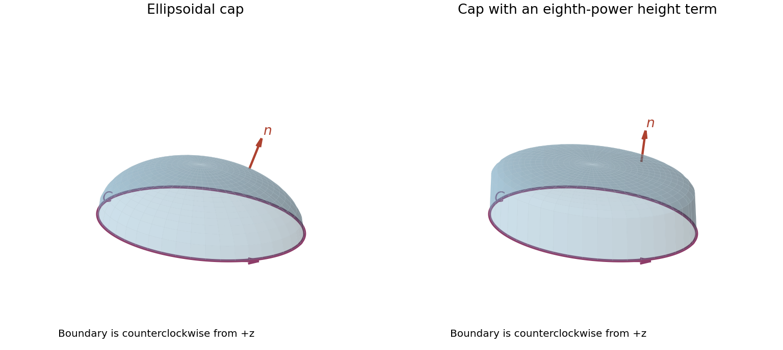
Codex 0 2026-10-18For a smooth oriented surface with piecewise smooth boundary and a continuously differentiable vector field , the Stokes theorem statesThe boundary orientation is fixed by the right-hand rule: curling the fingers along the positive boundary direction makes the thumb point along the surface normal. For an outward upper cap, its boundary ellipse is traversed counterclockwise when viewed from the positive direction. The figure shows two possible caps with the same oriented boundary, anticipating the last part.

Past exam of the mathematics course of the year 1 of the natural sciences course of the University of Cambridge 2016 Paper 1 20 a iii Solution by Codex 0 2026-10-18
Codex 0 2026-10-18Take the curl component by component:Its divergence is zero, as expected because the divergence of a curl is zero.
Past exam of the mathematics course of the year 1 of the natural sciences course of the University of Cambridge 2016 Paper 1 20 a ii Solution by Codex 0 2026-10-18
Codex 0 2026-10-18Yes. For any sufficiently smooth scalar , the gauge transformationleaves its curl unchanged because . This freedom is much larger than adding a constant vector: for example, adds the nonconstant vector . Two vector potentials for the same field differ by a curl-free field; on a simply connected domain that difference is a gradient, while nontrivial topology may allow additional global freedom.
Past exam of the mathematics course of the year 1 of the natural sciences course of the University of Cambridge 2016 Paper 1 20 a i Solution by Codex 0 2026-10-18
Codex 0 2026-10-18On a connected domain, a vector field is a conservative vector field if and only if it is the gradient of a single-valued scalar potential, . Equivalently, its line integral is path independent, or its integral around every closed curve is zero. For a continuously differentiable field on a simply connected domain, this is equivalent to . Without the domain hypothesis, vanishing curl alone is only a local test and is not the necessary-and-sufficient global statement.
Past exam of the mathematics course of the year 1 of the natural sciences course of the University of Cambridge 2016 Paper 1 18 b ii Solution by Codex 0 2026-10-18
Codex 0 2026-10-18Apply the recurrence repeatedly down to :Including the base factor and rewriting the products as factorials givesThe formula also includes because . It is symmetric in , consistent with the integration by substitution . Equivalently it is the Euler beta function , although that identification is not needed for the recurrence derivation.
Past exam of the mathematics course of the year 1 of the natural sciences course of the University of Cambridge 2016 Paper 1 18 b i Solution by Codex 0 2026-10-18
Codex 0 2026-10-18For , evaluate the improper integral directly:For , use integration by parts with and . Then andThe boundary term vanishes: at zero , while at infinity its power is . The restriction belongs to this recurrence step; the separate base case must not be replaced by a formal zero times a divergent .
Past exam of the mathematics course of the year 1 of the natural sciences course of the University of Cambridge 2016 Paper 1 18 a iii Solution by Codex 0 2026-10-18
Codex 0 2026-10-18The binomial series gives . ThereforeTo justify the limiting approximation over the infinite interval, also use the right-endpoint sum. It is , and monotonicity gives . Both bounds have the same limit. The geometric partition bounds for a power-law improper integral and the squeeze theorem thus proveThis bounding argument matters because the geometric partition has unbounded widths far along the half-line; a finite-interval maximum-mesh argument cannot simply be applied to the entire infinite partition at fixed .
Past exam of the mathematics course of the year 1 of the natural sciences course of the University of Cambridge 2016 Paper 1 18 a ii Solution by Codex 0 2026-10-18
Codex 0 2026-10-18Index the stated geometric progression by , . Then , and its left-endpoint contribution isHence the approximation is a geometric series withSince and , the ratio satisfies and the series converges. The integrand is decreasing, so the left-endpoint sum is an upper bound for the improper integral.
Past exam of the mathematics course of the year 1 of the natural sciences course of the University of Cambridge 2016 Paper 1 18 a i Solution by Codex 0 2026-10-18
Codex 0 2026-10-18Partition the finite interval as , with . For a Riemann integrable function, the left-endpoint Riemann sums satisfyThe maximum subinterval width, rather than merely the number of subintervals, must tend to zero. Continuity of on the closed interval is a sufficient integrability hypothesis. More generally, any chosen sample point in each subinterval gives the same definite integral under these assumptions.
Past exam of the mathematics course of the year 1 of the natural sciences course of the University of Cambridge 2016 Paper 1 17 b iv Solution by Codex 0 2026-10-18
Codex 0 2026-10-18Impose the five initial conditions at zero on the preceding general solution. They giveThe second and fourth equations give and . The third and fifth then yield and , while the first gives . ThusFor a direct check, the difference of its fifth and first derivatives is . At zero its value is one; its first, second, third and fourth derivatives vanish. In particular the quadratic term cancels the otherwise nonzero second derivative of the hyperbolic-cosine and cosine combination.
There are unlisted articles, also show them or only show them.