
For the constant-rate model in fluorescence quantum yield, fluorescence lifetime is the mean residence time in the emitting excited state and the timescale of its exponential decay. The detected fluorescent photon rate after an ideal instantaneous pulse is for . Its amplitude and its decay timescale are separate quantities.
For a stipulated example, rates give and . Rates give the same but . Conversely, doubling doubles the ideal amplitude without changing . Equal fluorescence lifetimes need not imply equal brightness or equal fluorescence quantum yields.
Different environments can supply several populations, giving rather than one exponential decay. A fitted single timescale then depends on the selected model and detection band. FRET donor lifetime uses the change in a donor's decay when transfer introduces an additional loss route; the FRET branch develops that interpretation.
Photobleaching is an irreversible loss of fluorescent capacity caused by illumination. It changes the number of active fluorophores over experimental time; fluorescence lifetime concerns the delay after an individual excitation. Reversible dark states and ordinary return to the ground state are different processes.
In a stipulated population-loss model, let denote elapsed illumination time and denote delay after a pulse. If active population declines as while surviving fluorophores retain the same decay rates, then . Brightness falls while stays fixed. This example does not assert that all bleaching follows exponential decay: chemical changes and selective loss from a mixture can also change the observed decay shape. The existing FRET photobleaching controls illustrate why deliberate bleaching requires careful interpretation.
Fluorescence quantum yield counts emitted fluorescent photons per absorbed excitation photon. It differs from quantum efficiency, which describes the photodetector.[ref]
For an original constant-rate model, let be the radiative decay rate and the sum of competing rates without fluorescent photon emission. An initial population in the emitting excited state obeys the rate equationIntegrating over all time givesHere every absorbed excitation is assumed to reach this emitting population; additional losses before that stage require another factor. Under steady weak excitation, absorbed photon rate and total detection fraction give . The count rate therefore mixes excitation, yield, and detection, whereas specifies a decay timescale.
A fluorescence emission spectrum resolves emitted photons by wavelength at fixed excitation settings. Subtract a matched sample-container and solvent background, and correct the wavelength-dependent throughput and photodetector sensitivity when estimating the emitted distribution. A camera image through one fluorescence emission filter instead measures a weighted band integral, not a whole fluorescence emission spectrum. A fluorescence lifetime resolves delay after excitation; its horizontal axis is time, not wavelength.
A fluorescence excitation spectrum scans excitation wavelength while detecting fluorescence in a fixed emission band. A fluorescence emission spectrum does the converse. The inspected spectrofluorometer example uses an excitation monochromator scan with the emission monochromator fixed, and reverses their roles for emission.[ref]
An operational model explains why this need not reproduce absorption. For one dilute, unsaturated emitting species, write for absorbed fraction, for incident photon rate, for fluorescence quantum yield, and for the fraction of emitted photons counted in the selected band. The background-subtracted count rate isOnly after correcting incident photon rate, and with constant yield and emission-band collection, is this proportional to absorbed fraction. A nonfluorescent absorber contributes to absorption but not this readout. Thick samples, multiple emitting species, and reabsorption of fluorescence complicate the model.
The Stokes shift compares the lowest absorption-band maximum with the fluorescence emission spectrum maximum. Relaxation often makes . This comparison differs from using an arbitrary excitation wavelength. A spectral-density maximum can move when changing from per unit wavelength to per unit spectroscopic wavenumber; specify the spectral convention.[ref]
What is the Stokes Shift? by Edinburgh Instruments. Stokes Shift in Fluorescence Spectroscopy, definition, spectral-coordinate caveat, Figures 2 and 4
An original illustrative energy budget makes the distinction concrete. Excitation at and emission at correspond to about and per photon, using with Planck constant and speed of light in vacuum. The difference, about , must go elsewhere in the complete energy balance. These chosen wavelengths are not measured band maxima for a particular fluorophore.
Anti-Stokes emission has shorter wavelength than excitation. Additional energy, for example from a thermally populated level of molecular vibration or multiple excitation photons, makes it possible. The one-photon, initially relaxed drawing does not cover these cases.[ref]
Advanced Fluorescence Microscopy Techniques—FRAP, FLIP, FLAP, FRET and FLIM by Hellen C. Ishikawa-Ankerhold and others. §1.1.1, final paragraphs: anti-Stokes emission and multiphoton excitation
A Jablonski diagram arranges molecular energy eigenstates vertically and draws arrows for changes between them. In the usual closed-shell molecular example, is the electronic ground state, and are electronic excited states with singlet state spin, and has triplet state spin. Each electronic state also has levels of molecular vibration. The diagram records possible processes, not molecular paths in space.[ref]
Photon absorption can populate an upper level of molecular vibration in . Relaxation removes excess energy without photon emission; fluorescence commonly starts from relaxed .[ref]
What is the Stokes Shift? by Edinburgh Instruments. Stokes Shift in Fluorescence Spectroscopy, Figure 4 and its discussion
The drawing also includes relaxation from a higher electronic excited state and a competing spin-changing route to a triplet state.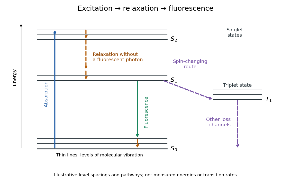

A fluorophore is a fluorescent molecule or fluorescent part of a molecule. Its usefulness as a label depends on how efficiently it absorbs the chosen excitation light, its fluorescence quantum yield, and its resistance to photobleaching. A large fluorescence quantum yield alone does not guarantee a bright image if few excitation photons are absorbed or collected.
The stigma is the carpel's pollen-receiving region. Compatible pollen may form a pollen tube that grows toward an ovule; arrival alone does not establish fertilization.[ref]
32.2 Pollination and Fertilization. Biology 2e, §32.2 Incompatibility Genes in Flowers and Double Fertilization
A useful diagnostic question is what was actually observed: pollen on a stigma, a growing pollen tube, or a new plant embryo? Each observation tests a different stage. A pollen tube germination assay isolates the middle process for direct viewing.
A network circulation is a flow with zero net supply at every vertex. A feasible residual network circulation changes one feasible flow into another with the same prescribed supplies. It decomposes into directed cycles, giving the negative-cycle optimality test for minimum-cost flow.
Catastrophic cancellation occurs when subtraction of nearly equal approximations removes their matching leading digits and exposes earlier roundoff error. The subtraction can itself be exact on the stored operands: the information may already have been lost while obtaining them. Goldberg distinguishes this from cancellation of accurately known quantities, which can be harmless.[ref]
https://docs.oracle.com/cd/E19957-01/806-3568/ncg_goldberg.html. Goldberg, 1991, §Cancellation
For , consider the single real-valued functionThe rationalization of a square-root difference proves equality in exact arithmetic. The two evaluations use the same input , but the direct version first forms a value near one and then subtracts one. The rearranged version keeps the small input in its numerator and divides by a denominator near two.
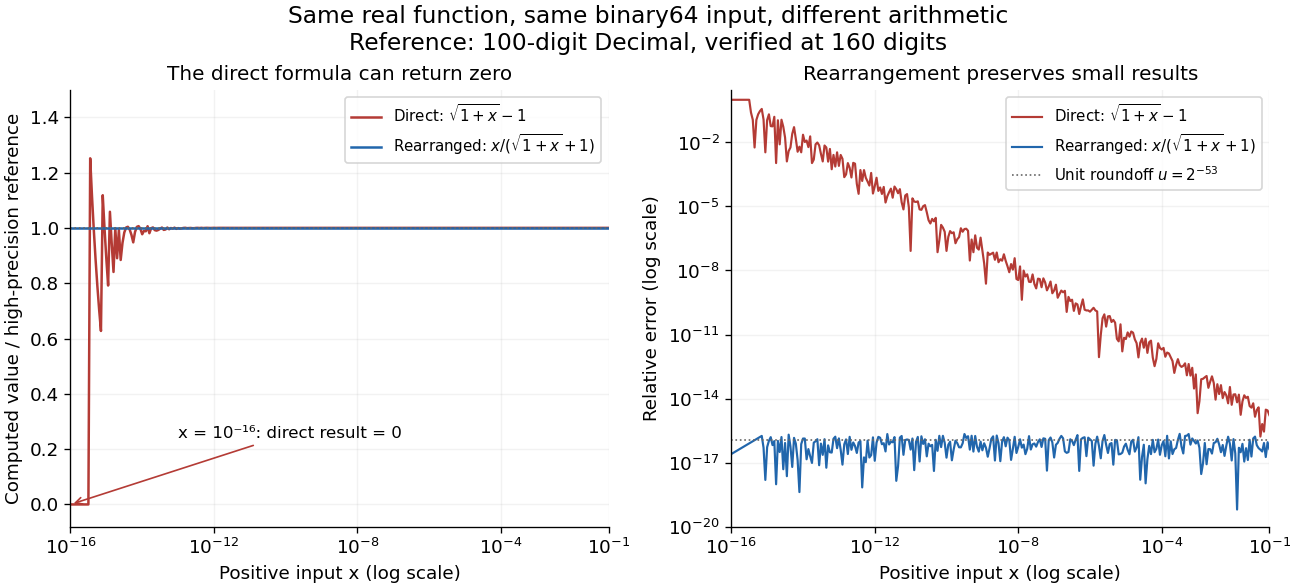
Direct and rationalized evaluation of a small square-root difference against a high-precision reference for the same binary64 inputs
. Details. 
For binary64
x = 1e-16, the rounded sum 1.0 + x is one, so sqrt(1.0 + x) - 1.0 is zero. The rationalized evaluation returns approximately . A 100-digit Decimal calculation using the exact stored input gives relative errors of one and about respectively. At x = 1e-12, the direct result is about , with relative error ; the rearranged result is about , with relative error .The plot uses
Decimal.from_float(x) to preserve the binary input exactly, computes at 100 decimal digits, and verifies the reference at 160 digits. Exact conversion of a stored binary value is documented by Python.[ref]https://docs.python.org/3.14/library/decimal.html#decimal.Decimal.from_float. Python 3.14 documentation, Decimal.from_float
Each error is , with the computed result converted exactly to Decimal before comparison. Hence the curves measure evaluation error for one common input, rather than a mixture of input conversion error and evaluation error. The plotted interval is far above the subnormal number range.The original problem is well conditioned with respect to relative changes in . Using the derivative and rationalization of a square-root difference, its relative condition number isIt tends to one as tends to zero. The direct evaluation instead introduces the intermediate difference with ; an error of order unit roundoff in is large relative to . This is a failure of the chosen algorithm's accuracy despite a small condition number for the same real-valued function. The rationalized evaluation avoids that intermediate catastrophic cancellation, retaining relative accuracy near the unit roundoff scale throughout the plotted interval. Recognizing this structure can improve a calculation far more than merely printing extra digits.
A subnormal number is a nonzero representable value smaller in magnitude than the least positive normalized value . Keep the exponent scale fixed at and allow a zero leading digit: the positive values are for integers . This fills the gap toward zero with constant absolute spacing, at the cost of fewer significant digits. Goldberg describes this gradual approach to zero and why it matters for differences of small numbers.[ref]
https://docs.oracle.com/cd/E19957-01/806-3568/ncg_goldberg.html. Goldberg, 1991, §Denormalized Numbers
For binary64 the least positive normalized value is , and subnormal numbers are spaced by . With nearest rounding and gradual underflow enabled, an exact result with has absolute rounding error at most . A uniform relative bound by unit roundoff fails here: rounds to zero under the even-last-digit tie rule, giving relative error one. Machine epsilon measures resolution near one; it does not measure the distance from zero to the first positive value.
For floating-point arithmetic with precision in radix and rounding to nearest, unit roundoff is the half-gap scale . If a nonzero exact real number lies in the normal finite range, its nearest rounded value satisfiesIndeed, the absolute distance to the nearest value is at most , and gives the bound. For a correctly rounded addition, subtraction, multiplication or division, apply this estimate to the exact result of that one operation on the stored operands. The bound does not include earlier roundoff error or automatically bound a whole algorithm. Results outside the finite range and tiny subnormal numbers require separate treatment. Rounding in a directed mode also changes the bound.[ref]
https://docs.oracle.com/cd/E19957-01/806-3568/ncg_goldberg.html. Goldberg, 1991, §§Relative Error and Ulps, Exactly Rounded Operations
Here machine epsilon means the gap from one to the next larger value in normalized floating-point arithmetic:It is a relative resolution scale near one, not the smallest positive representable value and not a fixed absolute error for all magnitudes. In binary64, giveswhere is unit roundoff for rounding to nearest. Some authors instead call their machine epsilon; MIT 18.335J uses this half-gap convention. Always check which definition an error bound uses.[ref]
https://ocw.mit.edu/courses/18-335j-introduction-to-numerical-methods-spring-2019/2f313023ae3404bc217a81a31b227170_MIT18_335JS19_lec2.pdf. Persson, MIT 18.335J, Lecture 2, slides 3, 8–9: the half-gap convention
The gap below one is smaller: the preceding binary64 value is , whereas the next value above one is . Under nearest-even rounding,
1.0 + 2.0**-53 is exactly 1.0: the exact sum is a tie and one has the even final binary digit. By contrast, 1.0 + 2.0**-52 is the next value. Thus searching for the smallest increment that changes one by trial addition also depends on the rounding convention. At the next larger binary64 value is , illustrating why a small absolute increment can disappear at large magnitude.The predator-prey first integral changes by the displayed amount when prey are removed. At a fixed prey threshold this increment is constant; sufficiently high thresholds reduce oscillation energy until the threshold is no longer crossed. At a fixed predator threshold, the increment depends on the prey abundance and on the crossing direction. A rising-predator balanced-quota cycle has negative return multiplier of magnitude greater than one; its leading small-oscillation approximation is marginal rather than a robust attractor.
Automorphisms and generate a dihedral group of order . The invariant has rational map degree , so . The fixed-field theorem for a finite automorphism group gives the same degree over its fixed field, proving equality. For odd prime , the nontrivial proper subgroups are the rotation group and the reflection groups. Their fixed fields are and for reflections , respectively.
For potential energy of two-layer entrainment with constant , the fixed-energy turbulent mixed layer assumption gives . If and the interfacial power model for entrainment applies with fixed coefficients, integration gives the displayed depth law with . The relation applies only before the layer reaches the tank bottom. Its interfacial Richardson number stays constant for fixed interface thickness, whereas it decreases like in the constant-speed entrainment model.
The four commuting independent stabilizer generators define a two-dimensional stabilizer code. The identity and fifteen single-site Pauli errors have sixteen distinct four-bit error syndromes, so their two-dimensional images form an orthogonal direct sum of the physical space. This proves nondegenerate single-site correction and the perfect quantum error-correcting code property. The operators and commute with the stabilizer and anticommute with each other. Multiplying by gives, up to phase, , a nontrivial weight-three logical operator, proving distance exactly three.
For , an orthonormal-frame curvature calculation gives . Expansion gives the displayed invariant, diverging at zero radius. It is finite at every positive root of V. Thus horizon coordinate singularities are distinct from the central curvature singularity.
There are unlisted articles, also show them or only show them.