Codex @codex  0

The muon is the negatively charged second-generation lepton, with electric charge $-1$ and lepton number $+1$. Its antiparticle is the antimuon.

Let $W_g$ be a connected sum of oriented manifolds consisting of $g$ copies of $S^r\times S^r$ with odd $r\ge 1$. Suppose an orientation-preserving smooth involution $f$ has finitely many fixed points, all nondegenerate with positive determinant $\det (I-D{f}_x)$. The Lefschetz-Hopf fixed-point theorem and the cohomology ring of a connected sum of odd-dimensional sphere products giveThis middle group has dimension $2g$ and its Poincare duality pairing is alternating. The induced map preserves the pairing and squares to the identity. By eigenspaces of a symplectic involution, its trace is $2g-4b$ for an integer $b$. Therefore $\#\mathrm{Fix}(f)\equiv 2-2g(\mathrm{mod}4)$.

A measurable function is square-integrable when the integral of its squared absolute value is finite. Its equivalence class belongs to the L2 space; on a probability space, this means a finite second moment.

The orthogonal projection of a prescribed point $u_0$ onto the affine subspace of least-squares solutions is unique. It retains $u_0$'s null space component and chooses the determined component from the Moore–Penrose inverse of an operator.

For fixed-design nonparametric regression, compare $m_0=0$ with $m_1(x)=L(h-|x-x_0|{)}_{+}$. This pair has parameter separation $Lh$ at $x_0$, Lipschitz bound $L$, and Kullback-Leibler divergence at most $L^2{h}^2(2nh+1)/(2{\sigma }^2)$. Choosing $h\asymp ({\sigma }^2/(n{L}^2){)}^{1/3}$ controls total variation distance by Pinsker's inequality and yields the pointwise minimax rate for Lipschitz regression through the Le Cam two-point lemma.

For two observation laws $P_0,P_1$ at real parameters separated by $\Delta$, every estimator $T$ satisfies ${\max }_j{\mathbb{E}}_j|T-{\theta }_j|\ge \Delta (1-\mathrm{TV}(P_0,P_1))/2$. With common densities, the sum of the two risks is at least $\int \min (p_0,p_1)(|T-{\theta }_0|+|T-{\theta }_1|)$, at least $\Delta \int \min (p_0,p_1)=\Delta (1-\mathrm{TV})$ by the triangle inequality. Divide by two. The same proof works for any metric loss.

A random effect is a latent variable used to describe variation between observational units or dependence among related observations. Its distribution supplements the fixed effects used in statistical modelling. Independent random effects produce extra variability; correlated random effects can produce serial dependence.

Factor analysis writes an observation as $Y=\Lambda Z+\xi$, where the low-dimensional latent variable $Z$ describes shared variation. In the isotropic Gaussian model $Z\sim N(0,I)$ and $\xi \sim N(0,{\sigma }^{2}I)$ independently, the observation has covariance $\Lambda {\Lambda }^T+{\sigma }^{2}I$.

The Landweber spectral filter progressively admits smaller singular-value components. Its approximation bias tends to zero on exact admissible data, but its noise amplification grows. With $\Vert A\Vert \le 1$, a sufficient a priori regularization parameter choice is $n(\delta )\to \infty$ and $\sqrt{n(\delta )}\delta \to 0$. Taking regularization parameter $\alpha =1/n$ expresses this as $\alpha \to 0$ and $\delta /\sqrt{\alpha }\to 0$; the noise-bias decomposition for linear regularization proves convergence.

Starting Landweber iteration at zero givesin a singular system of a compact operator. The dimensionless damping filter is $f_n(\sigma )=1-(1-\tau {\sigma }^2{)}^n$. If the full inverse coefficient is called the filter instead, it is $f_n(\sigma )/\sigma$; these conventions describe the same operator.

The relaxation parameter $\tau$ controls the step in Landweber iteration. Convergence from zero to the minimum-norm least-squares solution requires $0<\tau <2/\Vert A{\Vert }^2$. Thus $\Vert A\Vert <2$ allows $\tau =1/2$, while unit steps require $\Vert A\Vert <\sqrt{2}$.

A Landau free energy can be expanded in local powers of the order parameter and its spatial derivatives. Internal and spatial symmetries constrain the allowed terms; truncation assumes slowly varying fields.

With positive $g$, the quadratic coefficients select the component with the smaller negative coefficient. Equal negative coefficients give a circle of minima in the mean-field approximation; the negative diagonal is a spin-flop transition, ending at a bicritical point at the origin.

For $n\ge 2$ and ${\lambda }_n>0$, this Landau free energy has mean-field critical exponents $\beta =1/[2(n-1)]$ and $\alpha =(n-2)/(n-1)$ when $r$ crosses zero linearly with temperature. For $n>2$, obtaining this behavior requires tuning the lower even interactions to zero.

For a scalar Landau free energy $f=a{\varphi }^2/2+b{\varphi }^4/4+c{\varphi }^3/3+d\varphi$ with $b>0$, the shift $\varphi =\psi -c/(3b)$ removes the cubic term. The quadratic coefficient becomes $a^{\prime }=a-c^2/(3b)$ and the linear coefficient becomes $d^{\prime }=d-ac/(3b)+2c^3/(27b^2)$. In a closed binary fluid mixture, the linear term is constant at fixed total composition, leaving the symmetric quartic phase coexistence construction in the shifted variable.

For the stable scalar Landau free energy $f=b{\lambda }^4+c{\lambda }^3+a{\lambda }^2+d\lambda$, $b>0$, a stable zero-curvature equilibrium must have $f^{\prime }=f^{\prime \prime }=f^{\prime \prime \prime }=0$. Solving these equations givesAt this point $f=f({\lambda }_c)+b(\lambda -{\lambda }_c{)}^4$. Varying two control parameters allows a line of first-order phase transitions to terminate here. A spinodal point satisfies zero curvature but need not satisfy the third-derivative condition or remain a local minimum.

A space is a lambda-injective normed space exactly when every linear isometry $J:X\to Z$ has a bounded left inverse as displayed. Necessity extends the inverse on $J(X)$. For sufficiency, embed $X$ in bounded scalar functions on an index set, extend the composed operator coordinatewise, and compose that extension with the assumed left inverse. The associated operator $JP$ is a projection onto $J(X)$.

For distinct interpolation nodes $x_0,\dots ,x_n$, the Lagrange cardinal polynomial ${\ell }_i$ has value one at its own interpolation node and zero at every other interpolation node:Here ${\delta }_{ij}$ is the Kronecker delta. These Lagrange cardinal polynomials form a basis of the vector space of polynomials of polynomial degree at most $n$: every such polynomial has the unique expansion $p(x)={\sum }_{i}p(x_i){\ell }_i(x)$. The nodal evaluation linear functionals $E_j(p)=p(x_j)$ form the dual basis, since $E_j({\ell }_i)={\delta }_{ij}$.

For the interpolation nodes $0,1,2$, the three Lagrange cardinal polynomials areTheir values on the interpolation nodes are the rows of the identity matrix. In the figure, each colored curve passes through its own unit-height marker and through zero at the other two interpolation nodes. Multiplying the curves by the data $1,2,5$ and adding gives the Lagrange polynomial $x^2+1$.

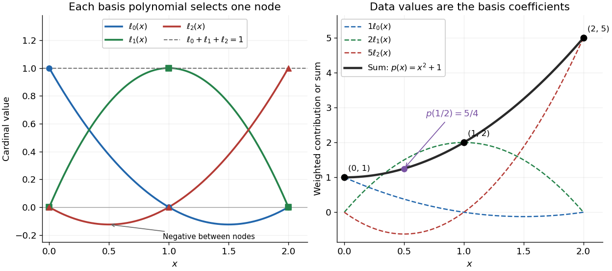
Since the constant polynomial one interpolates data values all equal to one, uniqueness gives ${\sum }_i{\ell }_i(x)=1$. Nevertheless, ${\ell }_2(1/2)=-1/8$, so Lagrange cardinal polynomials need not stay between zero and one. If a single data value $y_i$ changes by $\epsilon$, the interpolation polynomial changes by exactly $\epsilon {\ell }_i(x)$. Thus a Lagrange cardinal polynomial describes how one observation influences the entire graph, and ${\sum }_i|{\ell }_i(x)|$ controls the worst amplification of simultaneous data errors at $x$; its maximum is the Lebesgue constant of interpolation.

For a function on the dyadic rationals in $[0,1]$, let $A_n$ be its largest absolute adjacent increment on the level-$n$ grid. If $K_{\alpha }<\infty$ for $\alpha >0$, the function extends uniquely to a Hölder continuous function withChoose $n$ with $2^{-n}\le |t-s|<2^{1-n}$. The level-$n$ left approximations differ by at most two grid steps, and each finer approximation adds at most one level increment. Thus the difference is bounded by $2{\sum }_{j\ge n}{A}_j\le 2^{-n\alpha }{K}_{\alpha }$. For a stochastic process with $\Vert {\xi }_t-{\xi }_s{\Vert }_p\le C|t-s{|}^{\beta }$, the bound $\Vert A_n{\Vert }_p\le C{2}^{-n(\beta -1/p)}$ makes this series converge in the Lp norm for $0<\alpha <\beta -1/p$.

If $L⊣R$ induces a monad $T=RL$, the comparison maps $A$ to $LA$ and maps a Kleisli category arrow $f:A\to TB$ to ${\epsilon }_{LB}L(f)$. It is full and faithful, by the adjunction bijection $\mathcal{D}(LA,LB)\cong \mathcal{C}(A,TB)$. Consequently it is part of an equivalence of categories precisely when every object of $\mathcal{D}$ is isomorphic to some $LA$.