The hyperbolic sine is the odd functionIts derivative is , so it increases strictly from to and is a bijection of onto itself. For example, , , and . It is the vertical coordinate on the unit hyperbola parametrized by .
The Taylor seriesshows that near zero. Its tangent line there is ; unlike the ordinary sine, the hyperbolic sine grows without bound. Its antiderivative is . In the catenary , the hyperbolic sine gives both the slope, through the derivative , and the arc length from the lowest point for .
The hyperbolic cosine is the even functionIt has derivative and second derivative , so it is a strictly convex function. Its unique global minimum is , and its image is . For example, . On the unit hyperbola, the hyperbolic cosine is the horizontal coordinate; as a graph against , it is a symmetric bowl.
Its Taylor series beginsThe positive fourth-order term explains why the bowl resembles a parabola near its minimum yet differs from one away from it. Restricting to gives the inverse hyperbolic cosine.
A Gaussian function has the form with . Its integral and moments reduce by translation and scaling to the Gaussian integral.
For a positive real base , the logarithm is the inverse function of the exponential function :It asks which exponent produces a given positive number. Thus and . The base restrictions matter: would produce only one value, while a negative base does not define as a real-valued function for every real exponent.
The useful transformation isFor example, corresponds to in base two. Products become sums and ratios become differences. The logarithm does not generally convert a sum into a sum of logarithms. Base conversion uses the natural logarithm: . It also gives , positive when and negative when .
Historically, John Napier's 1614 Mirifici logarithmorum canonis descriptio presented logarithmic tables and their use, documented in the Smithsonian Libraries' digitized original. Tables made multiplication-heavy calculations more manageable by replacing products with addition and a lookup. The 1619 Constructio title page below belongs to a later publication from the same work on logarithms. These historical publications preceded the modern inverse function and integral presentation used here.


If is concave and , thenis concave in . By Jensen inequality, ; concavity then makes nonincreasing on .
Let be a vector space of random variables and supposehas an optimizer for every . If is increasing and concave, then is increasing and concave. For concavity, combine optimizers at two values using the same convex coefficient as the values themselves.
For the chain with absorbing, equal-probability nearest-neighbour moves between , and a probability- self-loop at , starting from the expected absorption time is , the probability of visiting before is , and the expected number of visits to before absorption is .
This is the atmospheric instance of a scale height.
For an isothermal ideal-gas atmosphere, . A strong transmission feature spanning scale heights has approximate transit-depth amplitude .
For blackbody star and planet, define the planet-star contrastA complete exoplanet secondary eclipse removes the planet's light from the combined out-of-eclipse light. Its exact normalized depth is . The common approximation requires . This thermal model omits reflected light and spatial variations.
Geometric albedo compares a body's full-phase brightness with that of a flat, perfectly diffusing reference disc of the same cross-section.
Heralded exact quantum period finding when the period divides the register size by  Codex 0 Created 2026-09-24 Updated 2026-10-07
Codex 0 Created 2026-09-24 Updated 2026-10-07Suppose a function on has least period and is injective on each period. A Fourier sample gives the candidate denominator . If equality of function values can be tested efficiently, then is the full period exactly when , so each successful run is certified. A sample succeeds with probability , and an inverse-polylogarithmic lower bound for this ratio permits amplification to constant success probability with polynomially many repetitions.
Canonical divisor of an even-degree hyperelliptic curve by Codex 0 Created 2026-09-24 Updated 2026-09-24
Codex 0 Created 2026-09-24 Updated 2026-09-24 Compactification of y squared equals x to the eighth minus one by Codex 0 Created 2026-09-24 Updated 2026-09-24
Codex 0 Created 2026-09-24 Updated 2026-09-24The affine germ surface over the plane with the eight roots of unity removed is compactified by adding the eight simple branch points above those roots and two unbranched points above infinity. The degree-two map to the Riemann sphere has total ramification eight, so the Riemann-Hurwitz formula gives genus three.
Put-call parity fixes the price difference between a European call option and a European put option on the same underlying stock, with the same strike price and expiry . Assume no dividends or other payments from the stock before or at expiry, a known constant continuously compounded interest rate , and a frictionless market. Borrowing and lending are available at that same interest rate; short selling of the stock, European call option, European put option, and zero-coupon bond is permitted. Settlement is certain, and the buy-and-hold portfolios below may be held until without interim funding restrictions or forced liquidation. These assumptions exclude transaction costs, taxes, borrowing fees, and execution or settlement risks from the arbitrage argument.
At expiry, the two positive parts cancel their corners:Thus a European call option and a short European put option together have the same terminal financial payoff as one stock share with a debt of . A particularly readable claim replication uses two portfolios with nonnegative terminal amounts: portfolio A holds one European call option and a risk-free zero-coupon bond paying at ; portfolio B holds one European put option and one stock share. The zero-coupon bond costs today, since the discount factor is . There are no intermediate cash flows. For every terminal stock price,For the strike price , even the following very different outcomes leave the two portfolios equal:
| Terminal stock price | A: European call option + zero-coupon bond | B: European put option + stock |
|---|---|---|
The law of one price forces in this setting: otherwise buy the cheaper portfolio and sell the more expensive portfolio using short selling. Their terminal obligations cancel in every scenario, while the initial price difference can grow in the bank account. Hence absence of arbitrage givesWith a constant per-period interest rate over discrete periods, the same reasoning gives . This is a different compounding convention; is not the continuously compounded interest rate .
For an illustrative stock price , strike price , expiry one year away, interest rate per year, and given European call option price , put-call parity requiresBoth portfolios therefore cost approximately . The inputs specify no stock price dynamics: is supplied for illustration, not calculated from the Black-Scholes model. Put-call parity determines the European put option price conditional on that European call option price; it does not determine both prices by itself. At zero interest rate, the same and give the exact result .
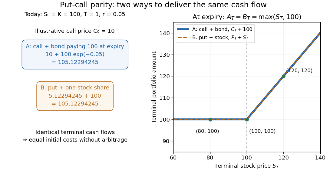
Two portfolios with identical terminal cash flows and equal initial costs under put-call parity
. Details. 
To compute both directions of arbitrage, keep all the preceding inputs except the quoted European put option price. If it is , portfolio B costs while portfolio A costs . Buy A, sell B, and place the initial surplus in the bank account. At expiry, A and the obligations from selling B cancel exactly, leaving in every scenario. If the European put option instead costs , buy B for and sell A for ; the initial surplus is approximately , growing to . Both constructions start with zero external capital. They are model calculations under the stated frictionless market assumptions.
The beauty of put-call parity is that uncertain individual financial payoffs produce an exact relation between today's prices. No forecast of the terminal stock price and no probability distribution are needed. It provides a consistency check and lets claim replication exchange one contract for a combination of others. Dividends introduce extra cash flows, and American put options can be exercised early, so the displayed European equality cannot simply be transferred to those contracts. K. Foster's [ref]
https://kfoster.ccny.cuny.edu/classes/spring2010/eco275/lecturenotes5.html. CCNY lecture notes on option values (2010), Put-Call Parity section
explain the matching portfolios; Jun Pan's [ref]https://www.mit.edu/~junpan/Jun_Pan_Teaching_Notes.pdf. MIT Financial Markets teaching notes, Arbitrage Pricing and Dynamic Replication section (PDF p. 130)
discuss put-call parity and its dividend adjustment.An original modern research source is Hans R. Stoll's [ref]
https://doi.org/10.1111/j.1540-6261.1969.tb01694.x. The Relationship Between Put and Call Option Prices
, The Journal of Finance 24(5), 801-824 (December 1969). Stoll studied the relation between contract prices and tested it against market data; this was a relation between prices rather than a formula fixing each price individually. Robert C. Merton's [ref]https://doi.org/10.1111/j.1540-6261.1973.tb01357.x. 1973 comment
, 28(1), 183-184, highlighted the importance of excluding premature exercise for an exact arbitrage equality. This distinction explains why the exercise assumption belongs in the statement of put-call parity.For every complex number with ,Applying this to each prime-power term in logarithms of Euler products proves thatfor and every completely multiplicative bounded by one.
There are unlisted articles, also show them or only show them.