Codex @codex  0

Given a family $A$ of approximating functions, a best uniform approximation to $f$ is an element $p\in A$ satisfying

Contracting two-mode oscillator bilinears with the Pauli matrices,gives $[T^a,T^b]=i{\epsilon }_{abc}{T}^c$. The subspace with total occupation $N$ is the spin-$N/2$ irreducible representation and has dimension $N+1$.

For bosonic modes satisfying $[a_i,a_j^{†}]={\delta }_{ij}$, the number-preserving bilinears $T_{ij}=a_i^{†}{a}_j$ obey

For the curvature conventionthe independent nonzero mixed components areand the Ricci scalar is $R=-2/a^2$.

Every radial coordinate line $\varphi =\text{constant}$ is a geodesic. No nonconstant coordinate circle $r=r_0>0$ is a geodesic.

As $x\to 0$, the limit $\sin x/x\to 1$ gives $\sin x\sim x$, while the Taylor series gives $\arcsin x\sim x$ and $\cos x\sim 1-x^2/2$.

These identities supply the formulas used in the tangent half-angle substitution. The half-angle identities include

The tangent is the trigonometric function $\tan x=\sin x/\cos x$ where $\cos x\ne 0$.

For a real angle $\theta$, $\cos \theta$ is the horizontal coordinate on the unit circle reached by a counterclockwise rotation through $\theta$ radians. For an acute angle in a right triangle, it is the adjacent side divided by the hypotenuse. Basic values includeAt $\theta =2\pi /3$, the horizontal coordinate is $-1/2$ even though the vertical sine coordinate remains positive. A positive angle need not produce a positive cosine.

Reflection across the horizontal axis leaves this coordinate unchanged, giving $\cos (-\theta )=\cos \theta$: cosine is an even function. A full turn gives $\cos (\theta +2\pi )=\cos \theta$. For real arguments, its range is $[-1,1]$ and its zeros of a function occur at $\theta =\pi /2+k\pi$. A quarter-turn shifts between the two coordinate traces, with $\cos \theta =\sin (\theta +\pi /2)$.

For a real angle $\theta$, $\sin \theta$ is the vertical coordinate on the unit circle reached by a counterclockwise rotation through $\theta$ radians. For an acute angle in a right triangle, it is the opposite side divided by the hypotenuse. In particular,The first-quarter rise and second-quarter fall are visible in the circle projection; the lower semicircle gives negative values.

Reflecting the unit circle across the horizontal axis gives $\sin (-\theta )=-\sin \theta$, so sine is an odd function. A full turn gives $\sin (\theta +2\pi )=\sin \theta$, making it a periodic function. For real arguments, its range is $[-1,1]$ and its zeros of a function occur at $\theta =k\pi$ for integers $k$. The cosine describes the perpendicular coordinate of the same point, and the Pythagorean trigonometric identity keeps their two values tied together.

Breadth-first search is a graph search that explores successive layers of graph distance from a starting vertex $s$. Here the graph is an undirected graph on a finite set of vertices, and distance counts edges, with no differing edge weights. Mark $s$ as discovered, assign $d(s)=0$, and place it in a FIFO queue. Repeatedly remove the front vertex $u$ and scan its adjacency list. Whenever a graph neighbour $v$ is still undiscovered, mark it immediately, record $u$ as its parent in a rooted tree in the discovery tree, assign $d(v)=d(u)+1$, and enqueue $v$ at the rear. Marking on insertion ensures that another edge cannot enqueue the same vertex again. ^[ref]

Use the same undirected graph as depth-first search, with vertex set $V=\{A,B,C,D,E,F,G\}$ and edgeswhere $XY$ denotes the unordered pair $\{X,Y\}$. Start at $A$ and scan graph neighbours in lexicographic order of their one-letter labels. The diagram's generator computes the following layers and the parent in a rooted tree assigned to each discovered vertex; the source is the root of a tree and has no parent in a rooted tree.

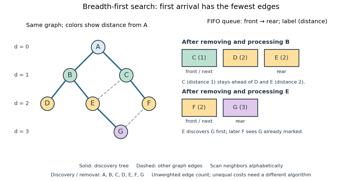
The discovery and removal orders both happen to be $A,B,C,D,E,F,G$. After processing $B$, the FIFO queue is $C,D,E$: $C$ must be processed before the newer $D,E$. Processing $C$ then skips the already discovered $E$ and enqueues $F$, giving $D,E,F$. Processing $D$ adds nothing. Processing $E$ discovers $G$, giving $F,G$; later $F$ sees $G$ already marked and leaves its parent in a rooted tree unchanged. The discovery edges are $AB,AC,BD,BE,CF,EG$, forming a rooted tree on all seven vertices even though the original graph contains graph cycles. The discovery tree contains six edges; it need not contain every examined edge.

First arrival is shortest because the FIFO queue keeps assigned distances in nondecreasing order, with entries from at most two consecutive layers. While processing distance $k$, newly discovered vertices receive distance $k+1$ and join the rear. If an undiscovered vertex had a shorter graph path, its preceding vertex on that graph path would lie in an earlier layer and would already have discovered it. Thus $d(v)$ is the minimum number of edges from $s$ to $v$. This is a mathematical induction over the layers, not an assumption about the drawing. Following the parent in a rooted tree backwards at each step gives $G,E,B,A$; reverse that sequence to obtain the three-edge graph path $A,B,E,G$. $A,C,F,G$ is another shortest graph path, but the specified graph neighbour order makes $E$ discover $G$ first. Changing that order can change the parent in a rooted tree without changing graph distances. ^[ref]

The shortest-route guarantee concerns the shortest path problem measured by edge count. It also minimizes total cost when every edge has the same positive cost. With unequal edge weights, first discovery need not minimize total cost; nonnegative costs can instead be handled by the Dijkstra algorithm. Breadth-first search is useful for minimum-hop routes and for finding all vertices within a specified graph distance. Its FIFO queue finishes an older layer before the next one, whereas depth-first search uses a call stack or explicit LIFO stack to pursue one branch immediately.

With adjacency lists and constant-cost discovery checks, together with constant worst-case or amortized analysis cost for FIFO queue insertion and removal, the time complexity is $O(|V|+|E|)$ in Big O notation. Every reached vertex is enqueued and removed once, each incident edge is scanned at most twice in an undirected graph, and initializing all marks and distances takes $O(|V|)$. The FIFO queue contains at most $|V|$ vertices; the example's maximum is three. Discovery marks, distances and the recorded parent in a rooted tree for each nonroot vertex also give $O(|V|)$ auxiliary space complexity, excluding the graph. An array that shifts every entry on front removal can lose the linear time complexity; the FIFO queue abstraction alone does not make removal constant-cost. Ordering the adjacency lists is a separate preprocessing cost.

A single start reaches only its connected component of a graph. Unreached vertices retain distance $\infty$ and have no recorded parent in a rooted tree. Restarting at each still-undiscovered vertex, while preserving all discovery marks, produces a forest covering the graph; each new root of a tree gets distance zero, so these distances refer to that root of a tree, not to the original $s$.

A spanning tree of a connected graph $G$ is a subgraph that is a tree and contains every vertex of $G$. Its edges must come from $G$. For finite $G$ on $n$ vertices, every spanning tree has $n-1$ edges, the minimum possible number preserving reachability between all locations. This makes a spanning tree a compact certificate that the original graph is connected. A minimum spanning tree additionally minimizes a specified total edge weight; merely selecting a spanning tree supplies no such optimization. ^[ref]

Let $G$ be our seven-vertex tree with edge $57$ added. It has seven edges and a graph cycle. Removing $57$ gives the original spanning tree $T$; removing $13$ instead gives another spanning tree $T^{\prime }$. Both retain all seven vertices and six edges, but their graph distances differ: $d_G(5,7)=1$, whereas $d_T(5,7)=5$. In $T^{\prime }$, $d_{T^{\prime }}(5,7)=1$ but $d_{T^{\prime }}(1,3)=5$, along $1,2,5,7,6,3$, compared with $d_G(1,3)=1$. Preserving reachability permits longer journeys; breadth-first search can preserve graph distances from one chosen starting vertex.

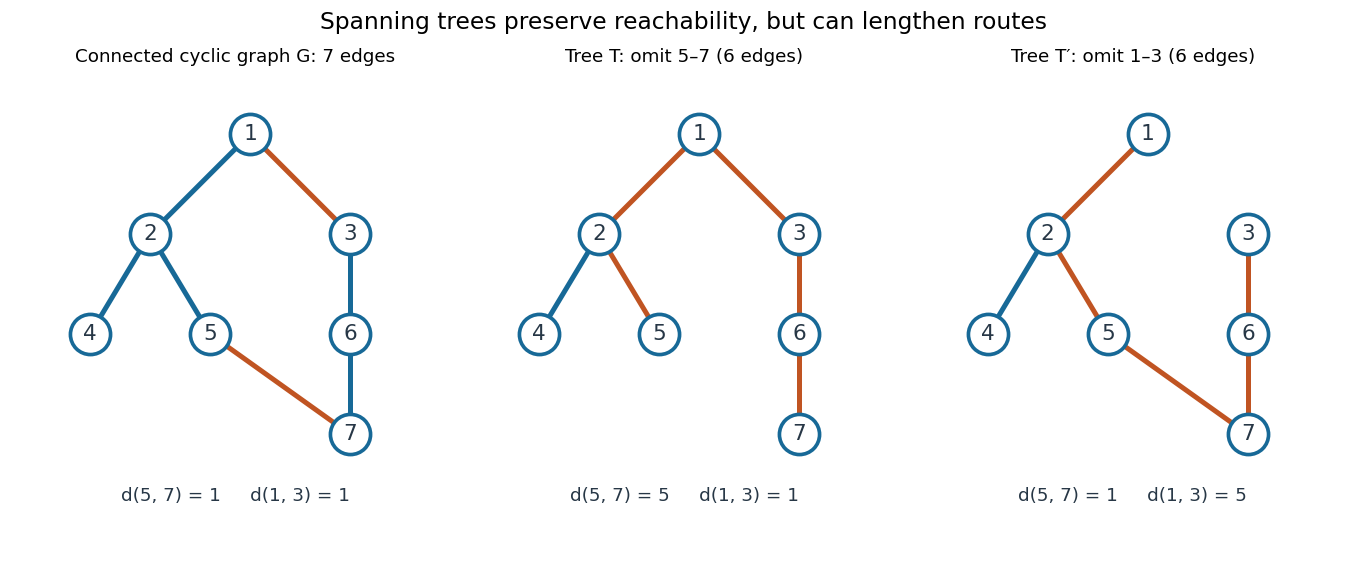
To construct a spanning tree, repeatedly delete any edge on a graph cycle. Its endpoints remain joined through the rest of that graph cycle, so the deletion preserves connectedness. Finiteness ensures that this stops at a connected acyclic graph. Conversely, adding an omitted edge to a spanning tree creates its unique fundamental cycle; deleting any other edge on that graph cycle produces another spanning tree. The displayed exchange replaces $13$ by $57$. ^[ref]

A forest is an undirected graph with no graph cycle; each of its connected components of a graph is a tree, including any isolated vertex. A finite forest with $n$ vertices and $c$ connected components of a graph hasIndeed, a connected component of a graph with $n_i$ vertices contributes $n_i-1$ edges; adding these counts gives $n-c$. Equivalently, start with $n$ isolated vertices: every added edge must join different connected components of a graph, reducing their number by one. Joining vertices already connected would create a graph cycle. ^[ref]

Deleting $13$ in our example gives $n=7$, $c=2$, and five edges: the two trees contribute $3+2=5=7-2$. Deleting $67$ as well leaves $7$ isolated, so $c=3$ and four edges. A forest therefore describes separate hierarchies or the intermediate stages of building a spanning tree. The acyclic graph condition accounts for missing connections without assuming that all locations are mutually reachable.

The linear spreading speed is obtained from exponentially decaying modes at an unstable state's leading edge and the condition that their spatial exponents become repeated.

The substitution $U(x,t)=U(x-ct)$ turns time derivatives into $-c{U}^{\prime }$ and spatial diffusion into $U^{\prime \prime }$, reducing a reaction-diffusion PDE to an ODE system.

Let $L$ be the open-loop transfer function. The winding of its Nyquist plot around $-1$, together with the number of unstable open-loop poles, determines the number of unstable zeros of $1+L$, which are the closed-loop poles.

A Liouville number admits rational approximations of every fixed polynomial order; Liouville's approximation theorem makes every such irrational number transcendental.

For any coupling of random variables, the coupling characterization of total variation distance gives $d_{\mathrm{TV}}(\mathcal{L}(X),\mathcal{L}(Y))\le \mathbb{P}(X\ne Y)$, where $\mathcal{L}$ denotes the law of a random variable. If two coupled Markov chains stay identical after their coalescence time $T$, then $\{X_t\ne Y_t\}\subseteq \{T>t\}$ andThe persistent agreement is essential: a first meeting time does not give this bound if the chains can separate again. A coalescing coupling turns a difficult comparison of probability distributions into a concrete question about how long a joint simulation takes to merge.

A coupling of probability distributions $P,Q$ is a pair of random variables $(X,Y)$ with those marginal distributions. On a finite set, and more generally on a standard Borel space, the least achievable mismatch isA maximal coupling attains the minimum; maximal here refers to agreement. An arbitrary coupling can have a much larger mismatch.^[ref]

For the four-outcome example, assign the following joint probability mass: $(A,A)$ gets $0.1$, $(B,B)$ gets $0.1$, $(C,C)$ gets $0.2$, and $(D,D)$ gets $0.3$. The remaining $0.3$ must have $X=A$; place $0.2$ on $(A,B)$ and $0.1$ on $(A,C)$. Row sums give $P$, column sums give $Q$, and the diagonal contains $0.7$. Agreement can reach 70%; mismatch cannot fall below 30%.

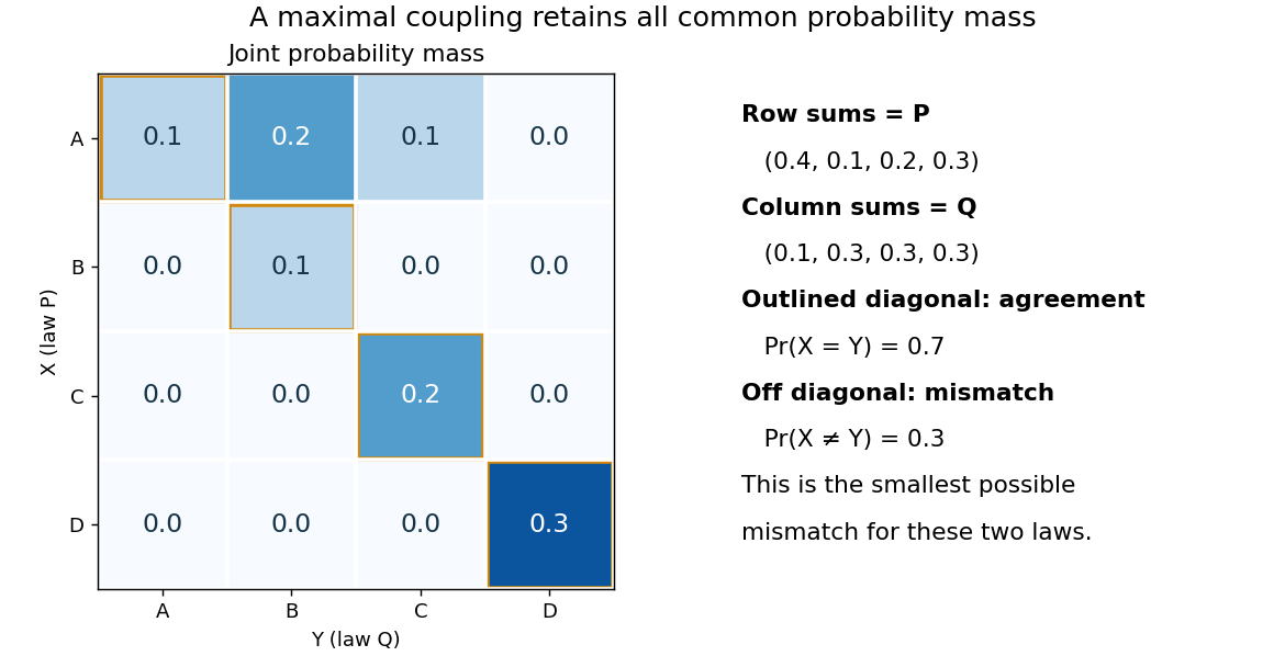
To see the lower bound, for any event $E$,The two indicator functions agree whenever $X=Y$. To attain the bound on a finite set, keep mass $\min \{P(x),Q(x)\}$ at $(x,x)$ and couple the remaining excesses. The two residual probability distributions live on disjoint subsets, so their part necessarily mismatches. When the probability distributions are identical, the residual part disappears entirely.

This is a choice of joint construction, not a claim that independently drawn observations are usually equal. Two independent random variables with the same continuous probability distribution can disagree with probability one even though their total variation distance is zero. The construction of a maximal coupling deliberately introduces statistical dependence to reveal how similar the marginal laws are.

If three closed sets cover a triangle and respectively contain its three opposite sides, then their triple intersection is nonempty.