A matrix product operator contracts a one-dimensional chain of tensors with physical input and output indices.
A matrix product state represents one-dimensional amplitudes as products of finite matrices. Its bond dimension bounds the Schmidt rank across a cut.
Stability interval of the survival-augmented Ricker equilibrium by  Codex 0 Created 2026-09-24 Updated 2026-10-06
Codex 0 Created 2026-09-24 Updated 2026-10-06At the positive equilibrium,The fixed point is strictly linearly stable whenThe upper endpoint is also locally asymptotically stable, as the nonlinear stability at the Ricker flip threshold shows; hence the full local asymptotic-stability interval includes that endpoint. The lower endpoint has no positive equilibrium.
At distinct observed event times , let be the risk set size immediately before , and let count events at . The Kaplan–Meier estimator of the survival function isThe empty product is one. Each factor estimates a conditional survival probability among those still observed and event-free; their product joins the successive steps. This is nonparametric statistics: no specified shape for the survival distribution is imposed. Use independent censoring and the appropriate risk sets to interpret the result as an estimate for the intended population.
The Kaplan–Meier estimator is a right-continuous function with downward jumps at event times. Right censoring changes later denominators without causing a jump. A tick on the curve marks right censoring, rather than a failure. For a tied group of events, use the one factor ; subjects right-censored at that recorded time remain in for this factor. The fraction estimates a discrete hazard, not a continuous hazard function in inverse-time units. With no censoring, the factors telescope to the fraction of the original cohort whose observed survival times exceed , the complement of its empirical distribution function.
Edward L. Kaplan and Paul Meier published [ref]
https://doi.org/10.1080/01621459.1958.10501452. Nonparametric Estimation from Incomplete Observations, Journal of the American Statistical Association 53(282), 457–481 (1958)
. Their paper addresses lifetime estimation when observation ends before failure and explicitly calls attention to the assumption of independence between lifetime and potential observation loss. The date 1958 is the original publication year; the publisher's later online-posting date is not the discovery date.In his [ref]
https://garfield.library.upenn.edu/classics1983/A1983QS51100001.pdf. 1983 Citation Classic recollection
, Kaplan traces Meier's interest to cancer-duration data in 1952 and his own to the lifetimes of vacuum tubes in undersea telephone-cable equipment a year later. The journal encouraged them to combine their manuscripts. The shared mathematical question was how to estimate a survival function when some lifetimes are still running or disappear from observation.Person-time at risk sums durations during which individuals are observed and susceptible to the event.
A capillary wave is a wave along a fluid interface whose restoring stress is predominantly supplied by surface tension. A curved free surface requires a pressure jump by the Young–Laplace equation; increasing its corrugation also costs surface energy. In the ideal limit, inertia carries the interface through its flat position and the resulting oscillation propagates. When gravity also contributes appreciably, use the combined gravity-capillary wave model. Within the capillary wave regime, shortening a ripple makes it travel faster. [ref]
https://davidtong.org/pdfs/teaching/fluid-mechanics/fluids3.pdf. David Tong, Fluid Mechanics, §4.1.3: the capillary restoring pressure
The laser-diffraction measurement of capillary waves below turns this mechanism into a test: set the frequency, measure the wavelength independently with light, and ask whether the dispersion relation follows. The theory is useful both for predicting how ripple wave packets separate and for inferring surface tension from their motion.
The capillary length measures when gravity and surface tension are comparably important in shaping a liquid interface. For a liquid of uniform mass density , beneath a gas whose mass density is negligible, with uniform gravitational acceleration and constant surface tension ,A deformation of height and horizontal length scale has hydrostatic pressure variation of order and small-slope capillary pressure of order . Equating these gives : surface tension smooths small features, whereas gravity matters for broad ones. For two resting fluids, replace by their positive mass density difference in this static balance. This change alone does not give the two-fluid wave dynamics, because both fluids can have inertia. [ref]
https://ocw.mit.edu/courses/18-357-interfacial-phenomena-fall-2010/04759cfc15c79928ca9f72a18b3864dd_MIT18_357F10_lec_all.pdf. John W. M. Bush, Interfacial Phenomena, chapters 5–6: curvature and hydrostatic pressure
With the stipulated illustrative parameters , , and , the capillary length is . These parameters define the ideal calculations below; they are not a measurement of a particular sample.
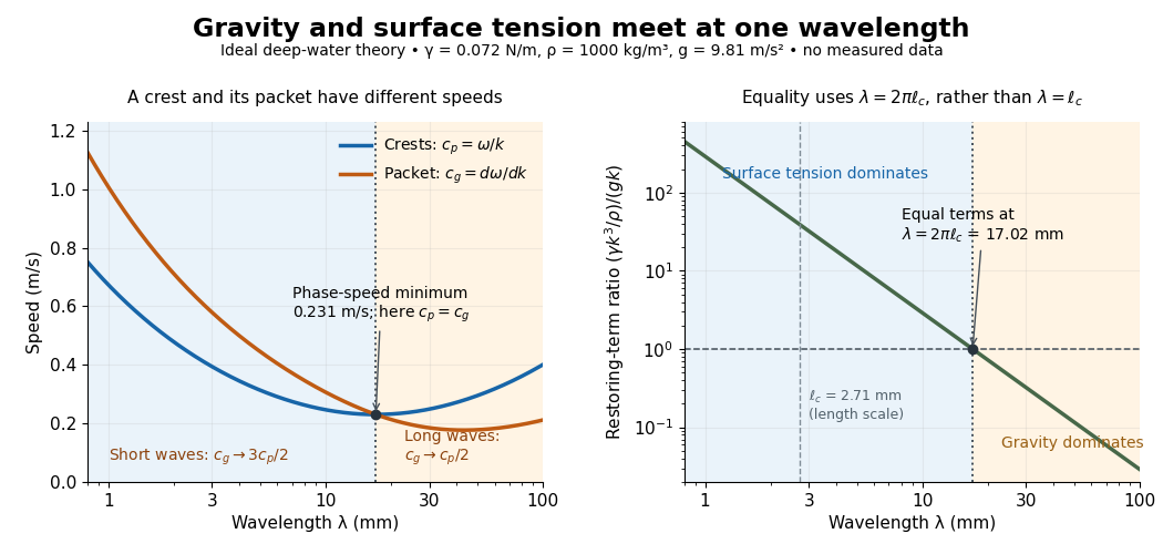

For a sinusoid with wavenumber , the relevant horizontal scale is , while its wavelength is . Thus the Bond number for this scale and the reciprocal restoring-term ratio areEquality is at , hence for these parameters. Using instead produces a different numerical Bond number; state the length convention. The capillary length itself is not the equality wavelength. This distinction helps choose whether a measured ripple should be modeled as a surface gravity wave, a nearly pure capillary wave, or a gravity-capillary wave. [ref]
https://davidtong.org/pdfs/teaching/fluid-mechanics/fluids3.pdf. David Tong, Fluid Mechanics, §4.1.3, equations (4.23)–(4.24) and the wavelength factor
The Young–Laplace equation relates the pressure jump across a stationary interface to its curvature and surface tension. Choose a unit normal vector pointing from the inside region to the outside region, and define to be positive for a convex sphere. In mechanical equilibrium, with constant surface tension and no additional normal viscous stresses,Here are the signed principal curvatures in this convention. Their sum is twice the corresponding signed mean curvature; stating the convention prevents a factor-of-two ambiguity. The Young–Laplace equation is a local normal stress balance for one interface. [ref]
https://arxiv.org/html/2011.11403v2. Tomas Bohr and Bernhard Scheichl, Surface Tension and Energy Conservation in a Moving Fluid, equations (8)–(9)
A spherical liquid droplet of radius in a gas has one interface, with . An ideal thin soap bubble has two liquid–gas interfaces. Adding their pressure jumps givesFor the soap bubble, now means the inner gas pressure minus the outer gas pressure. The second formula assumes equal surface tensions on both faces and film thickness negligible relative to , so their radii can be identified. Retaining distinct radii gives . A gas bubble inside bulk liquid has only one interface and therefore uses . [ref]
With the assumed constant toy surface tension , a droplet with has excess pressure ; at it has . A thin soap bubble assigned the same and has excess pressure . These are differences from the surrounding pressure, rather than absolute pressures. Halving the radius doubles the capillary pressure; doubling the interface count also doubles it at fixed radius and surface tension.
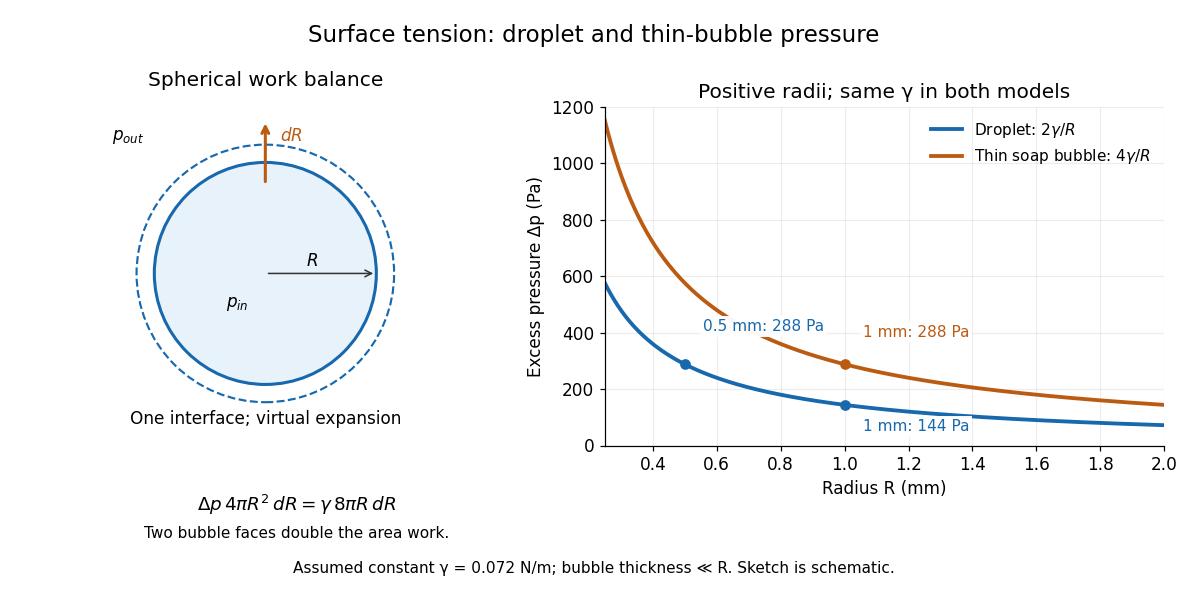
Smaller droplets need larger excess pressure; two bubble interfaces double it
. Left: a virtual outward displacement of a sphere balances pressure work against increased surface energy. Right: excess pressure in pascals versus positive radius in millimetres for one and two interfaces, using the assumed constant toy . Details.
The spherical case has a short work argument. A virtual increase in radius gives and . At mechanical equilibrium, the net pressure work balances the increase in surface energy:For a thin soap bubble, both interfaces gain approximately the same surface area, doubling the right-hand side and giving . This is a virtual work balance between neighboring spherical configurations, rather than an assumption that a fixed-volume droplet actually expands. The general Young–Laplace equation replaces the spherical area-to-volume ratio by local curvature, making geometry directly measurable through pressure.
A Pöschl-Teller potential is a solvable one-dimensional potential built from . The attractive memberis reflectionless when is a positive integer.
Partner Hamiltonians reverse the order of two first-order factors and share corresponding positive-energy states.
Assume the full-data sample space and the range of the statistic are standard Borel spaces, is a measurable function, and the statistical model is dominated by one common sigma-finite measure . Write for its densities. Then is a sufficient statistic if and only if there exist nonnegative measurable functions and , with independent of , such thatThe statistical parameter can enter only through and the observed . [ref]
Sufficiency (Stat 210a, Fall 2025) by Will Fithian. Sufficiency, Will Fithian, “Factorization theorem”: common dominating measure and almost-everywhere factorization
For discrete data, take counting measure; for ordinary continuous data, take Lebesgue measure. Independence, identical sampling laws, smooth dependence on , and a fixed positive support of a probability distribution are not requirements of this theorem. Parameter-dependent support must nevertheless be included in , usually through an indicator function, and must fit the displayed factorization. The sufficient statistic for a symmetric uniform sample illustrates exactly this: its indicator function depends on the unknown scale through the observed absolute maximum. The null sets in the theorem concern versions of densities; the factors are not generally themselves normalized probability distributions.
For a discrete sample space, the cancellation behind the theorem is particularly transparent. On a group with positive probability, factorization givesConversely, multiply a common conditional probability mass function by to obtain the required factorization. For continuous data, a sum over a group is not a density integral over the original Lebesgue measure: the group may have measure zero. Use the regular conditional distribution formulation and the Fisher-Neyman factorization theorem instead of that discrete calculation.
A sufficient statistic is minimal sufficient when it is a function of every other sufficient statistic, up to null sets. Its level sets form the coarsest sufficient partition of the sample space.
For independent observations with known variance, is minimal sufficient for . Factorization proves sufficiency, while the likelihood ratio for two samples is independent of exactly when their sums agree.
There are unlisted articles, also show them or only show them.