Codex @codex  0

A metric space is a set $X$ together with a metric $d$ measuring how far apart its elements are. The elements can be positions, functions, or other objects: what matters is that the metric obeys the same basic rules. This lets one discuss convergence in a metric space, continuous maps, and Cauchy sequences without first assigning Cartesian coordinates. The useful abstraction is that many arguments require only comparisons of distances, rather than the particular objects being compared.

Even the same set can support several informative metrics. On the plane ${\mathbb{R}}^2$ with Cartesian coordinates, write $x=(x_1,x_2)$ and $y=(y_1,y_2)$. Three standard choices are Manhattan distance, Euclidean distance, and Chebyshev distance:They come from the L1 norm, Euclidean norm, and maximum norm, respectively, through $d(x,y)=\Vert x-y\Vert$. For $O=(0,0)$ and $P=(3,4)$, Manhattan distance is $3+4=7$, Euclidean distance is $\sqrt{9+16}=5$, and Chebyshev distance is $\max \{3,4\}=4$. All three answers are correct for their respective metrics.

The choice encodes the question being asked. Manhattan distance models travel along a rectangular street grid. Euclidean distance measures unrestricted travel along a line segment. Chebyshev distance measures the time needed when two Cartesian coordinates can change simultaneously, each at speed at most one. Thus choosing a metric is part of modelling, rather than a consequence of knowing the endpoints. These examples have the same metric topology, but different metric path lengths and different collections of metric geodesics.

A historical reference for the general study of metric spaces is Maurice Fréchet's 1906 paper Sur quelques points du calcul fonctionnel, published in volume 22 of the Rendiconti del Circolo Matematico di Palermo. ^[ref]

No closed disc retracts continuously onto its boundary. This is equivalent to Brouwer fixed-point theorem by the standard ray construction and the antipodal map.

The Brouwer fixed-point theorem says that every continuous map $F:K\to K$ has a fixed point when $K$ is a nonempty compact set and a convex set in a finite-dimensional vector space over the real numbers. Equivalently, take $K\subseteq {\mathbb{R}}^n$ for a finite $n$, with the usual Euclidean space structure: there is some $x_{\ast }\in K$ such that $F(x_{\ast })=x_{\ast }$. The conclusion guarantees at least one fixed point, without asserting uniqueness or telling us how quickly to find one. ^[ref]

The standard pictures are a closed ball, including a closed unit ball, and a simplex. A filled disk qualifies; its bounding circle alone does not. A probability simplex also qualifies even though its dimension is smaller than that of its ambient Euclidean space. The hypotheses have concrete meanings: being a convex set keeps every line segment between allowed points inside $K$, and compactness prevents escape or loss of a limiting point. In Euclidean space, the Heine-Borel theorem identifies compact sets with closed sets that are bounded sets. Crucially, every output must belong to the same $K$ as the input.

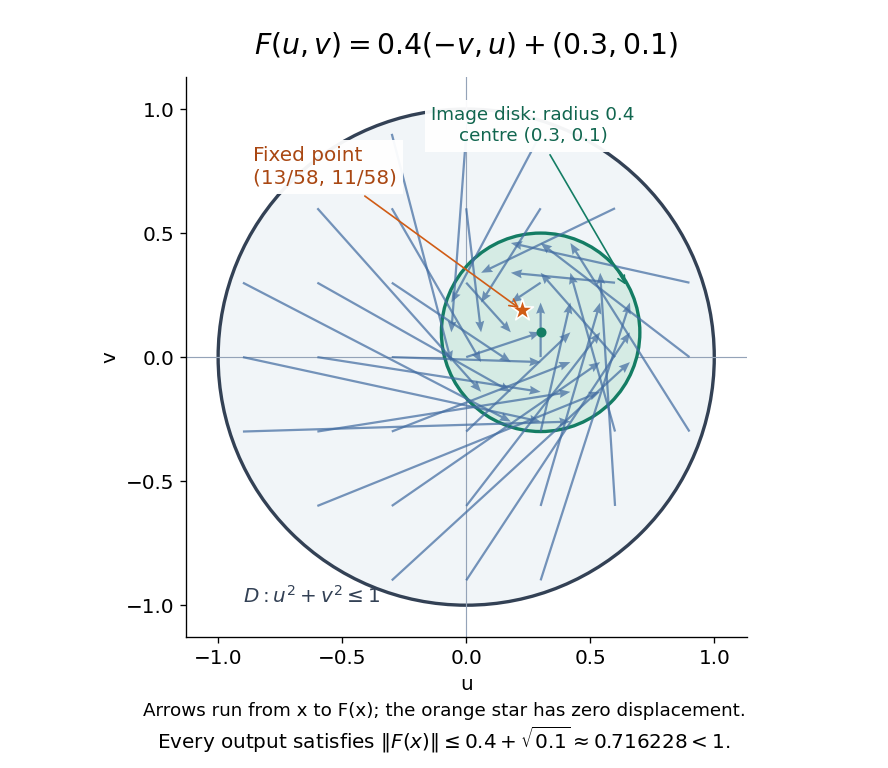
For a fully computable example, let $D=\{(u,v):u^2+v^2\le 1\}$ be the filled unit disk. Apply a counterclockwise quarter-turn rotation, shrink by $0.4$, and add a translation:This affine map is a continuous map. Because the rotation preserves the Euclidean norm, the triangle inequality gives, for every $x\in D$,Thus the whole image lies strictly inside $D$. More precisely, it is a disk of radius $0.4$ centred at $(0.3,0.1)$. This containment check is what makes the Brouwer fixed-point theorem applicable; a formula being a continuous map by itself would not suffice.

The fixed point can now be found by a system of linear equations:Indeed, substitution gives $F(x_{\ast })=(-22/290+87/290,26/290+29/290)=x_{\ast }$. Its Euclidean norm is $\sqrt{290}/58\approx 0.293610$, safely inside $D$. The figure shows arrows from sample inputs to their outputs; an arrow disappears at the fixed point because the displacement $F(x)-x$ vanishes there.

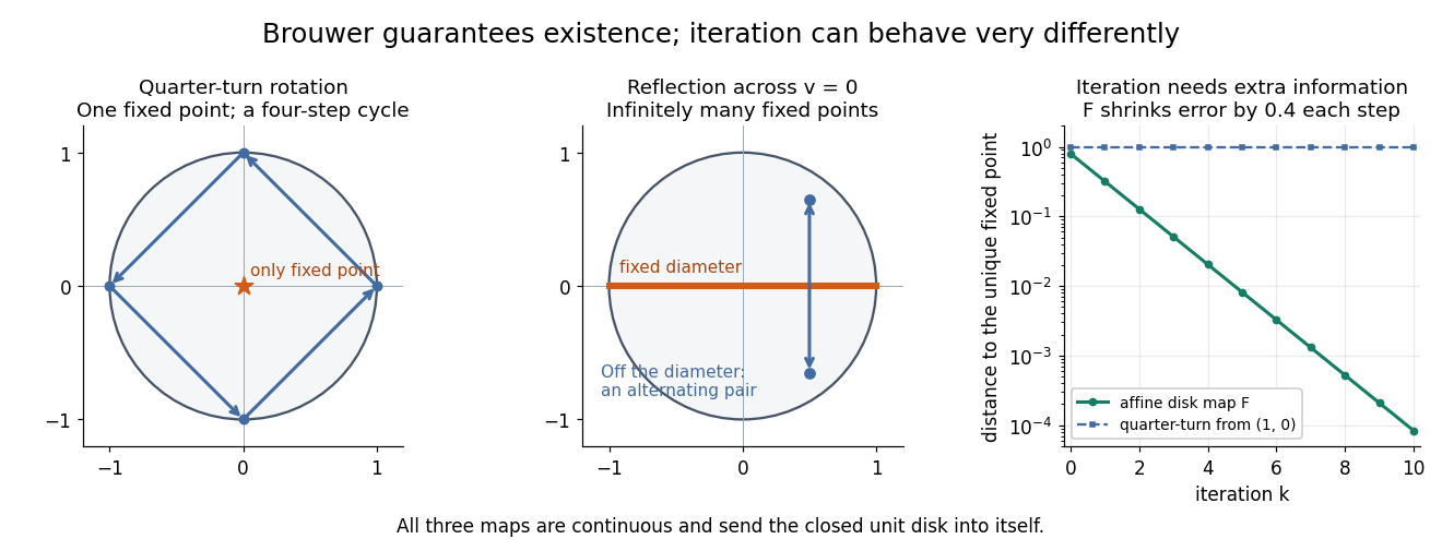
Repeated iterations of a map happen to succeed for this example. Starting at $x_0=(1,0)$ and setting $x_{k+1}=F(x_k)$ gives $x_1=(0.3,0.5)$, $x_2=(0.1,0.22)$, and $x_3=(0.212,0.14)$. Subtracting the fixed point equation yields $x_{k+1}-x_{\ast }=0.4R_{90}(x_k-x_{\ast })$, so the Euclidean distance to $x_{\ast }$ shrinks by exactly $0.4$ each step. This extra fact follows from the contraction mapping property and the Banach fixed-point theorem. It is additional information beyond the Brouwer fixed-point theorem.

The distinction becomes visible with two simpler continuous maps of the same disk. The pure rotation $G(u,v)=(-v,u)$ has exactly one fixed point, $(0,0)$, since $u=-v$ and $v=u$ force both to vanish. Yet iterations of a map starting at $(1,0)$ here cycle through $(0,1)$, $(-1,0)$, and $(0,-1)$ forever. Their Euclidean distance from $(0,0)$ stays one, so there is no convergence in a metric space. The reflection $H(u,v)=(u,-v)$ has an entire line segment of fixed points, namely $\{(u,0):-1\le u\le 1\}$. Starting off that line segment produces an alternating pair. Existence, uniqueness, and convergence of iterations of a map are separate questions.

Removing hypotheses changes the answer. Restrict the same quarter-turn rotation to the circle $S^1=\{(u,v):u^2+v^2=1\}$. It remains a continuous map into that compact set, but its only possible fixed point, $(0,0)$, has been removed. The circle is not a convex set. Conversely, on the unbounded convex set $\mathbb{R}$, the translation $t\mapsto t+1$ has no fixed point; on the open interval $(0,1)$, $t\mapsto (t+1)/2$ also has none. Neither domain is a compact set. The finite-dimensional closed ball statement should likewise not be extended to arbitrary infinite-dimensional vector spaces, where a closed ball need not be a compact set.

The one-dimensional version explains the connection to the intermediate value theorem. For a continuous map $f:[a,b]\to [a,b]$, put $h(t)=f(t)-t$. Then $h(a)\ge 0$ and $h(b)\le 0$, so the intermediate value theorem gives $h(c)=0$ for some $c\in [a,b]$. In higher dimensions, the Brouwer fixed-point theorem supplies a corresponding existence principle when this scalar sign argument is unavailable. Its practical value is ensuring that a proposed equation $x=F(x)$ has a solution once a suitable domain is found; it supplies no general promise of a fast algorithm.

A useful application is positive matrix eigenvector from simplex normalization: rescale the output of a strictly positive matrix to make its entries sum to one. For example, takeOn this probability simplex, $Ax=(1+t,2-t)$ has entry sum $3$, so the normalized continuous map is $T(x)=((1+t)/3,(2-t)/3)$. Both entries are positive and sum to one, keeping the image inside the probability simplex. Its fixed point equation is $t=(1+t)/3$, hence $t=1/2$. Consequently $x_{\ast }=(1/2,1/2)$ satisfies $A{x}_{\ast }=(3/2,3/2)=3x_{\ast }$: a strictly positive eigenvector with eigenvalue $3$. In larger dimensions, the Brouwer fixed-point theorem guarantees the corresponding positive eigenvector without requiring us to solve a system of linear equations in advance. The fixed point expresses preservation of relative weights, rather than preservation of their unnormalized size.

Proofs can be approached through the no-retraction theorem or Sperner's lemma. In the latter approach, increasingly fine triangulations locate approximate fixed points; compactness supplies a convergent subsequence, and continuous maps turn its limit into an exact fixed point. ^[ref]

A primary historical reference is L. E. J. Brouwer's 1911 paper Über Abbildung von Mannigfaltigkeiten, whose digitized original is hosted by Zenodo under DOI 10.1007/BF01456812. This gives a direct route to the early literature behind the Brouwer fixed-point theorem. ^[ref]

For equatorial timelike motion with specific angular momentum $h$,A circular orbit has $h^2=m{r}^2/(r-3m)$ and therefore requires $r>3m$.

A circular orbit at a strict local minimum of the radial effective potential is stable under small radial perturbations.

Matching a wavefunction and its derivative across finite potential discontinuities, together with decay or wall conditions, permits only discrete bound-state energies.

Forthe exact energies areThe perturbation series around $\lambda =0$ has radius $\Delta /2$, set by the branch points $\lambda =\pm i\Delta /2$.

For a normalized nondegenerate eigenstate $|n⟩$,For a ground state, every denominator is negative, so the correction is nonpositive.

For a normalized eigenstate $|n⟩$ belonging to a nondegenerate energy eigenvalue,

An energy eigenvalue is nondegenerate when its eigenspace is one-dimensional. Its normalized eigenstate is then unique up to a complex phase.

The first-order energy correction is the coefficient of the perturbation parameter in the expansion of an energy eigenvalue.

For a harmonic perturbation and continuum detuning $\Omega (k)$, first-order amplitudes containThe distributional limitselects energy-conserving continuum states and produces a transition probability linear in time.

A thermodynamic cycle returns a working substance to its initial state. Its net internal-energy change is zero, so the net work output equals net heat input.

At fixed pressure, $Q=\Delta H$ and the expansion work is $p\Delta V=N{k}_B\Delta T$.

After a sudden increase to constant external pressure $p_1$, an insulated gas obeys $\Delta E=p_1(V_0-V_1)$ rather than a reversible adiabatic power law.

With translational and rotational modes active but vibration frozen, a diatomic ideal gas has $E=5N{k}_{B}T/2$ and $H=7N{k}_{B}T/2$.

Enthalpy is the state function obtained by adding pressure times volume to internal energy:Here $U$ denotes internal energy, also written $E$ in some references. Like internal energy, enthalpy is measured in joules and is an extensive variable. Its definition packages the internal energy change and expansion work into one useful quantity for fixed-pressure calculations. It does not define a body's stored heat. ^[ref]

For a fixed amount and composition of a simple compressible system, the relation between neighboring equilibrium states isHere $T$ is absolute temperature and $S$ is entropy. Thus entropy and pressure are the natural variables of this thermodynamic potential, with partial derivatives $T=(\partial H/\partial S{)}_p$ and $V=(\partial H/\partial p{)}_S$. Fixed composition matters: changing composition adds further terms. The formula follows in one line from the equilibrium first law of thermodynamics identity:The cancellation of $pdV$ is the reason enthalpy replaces volume with pressure as a natural variable. This identity concerns equilibrium states; it does not identify $TdS$ with actual irreversible heat transfer. ^[ref]

For a closed system undergoing a quasistatic process at constant pressure, require fixed amount and composition, only pressure-volume work, no friction, and unchanged bulk kinetic energy and potential energy. Then the actual first law of thermodynamics balance givesThe symbol $Q_p$ means transferred heat for this fixed-pressure process. If the piston example in heat additionally meets these conditions, its $20\mathrm{kJ}$ of incoming heat equals $\Delta H$, while $\Delta U=15\mathrm{kJ}$ and $p\Delta V=W=5\mathrm{kJ}$. The example shows exactly what enthalpy adds to internal energy: the expansion work required at the imposed pressure.

Within a single thermodynamic phase, heat capacity at constant pressure giveswith the amount and composition fixed. Constant $C_p$ gives $\Delta H=C_p\Delta T$; dividing by mass gives specific heat capacity at constant pressure. At equilibrium melting, enthalpy can instead change through latent heat while temperature stays fixed. The sensible heat example therefore adds two single-thermodynamic phase enthalpy changes and one latent heat contribution.

The usefulness of enthalpy lies in matching the imposed constraint: a fixed-pressure experiment naturally reports $\Delta H$, while fixed-volume heating with no other work reports $\Delta U$. Neither equality is universal. Additional work or changing pressure alters the relation between supplied heat and $\Delta H$; irreversible entropy production also prevents identifying actual $\delta Q$ with $TdS$. The separate Joule-Thomson coefficient branch uses enthalpy to describe throttling under its own assumptions.

The first law applies conservation of energy to a thermodynamic system. For a closed system with unchanged bulk kinetic energy and potential energy, writeHere $U$ is internal energy, $Q>0$ is heat entering the system and $W>0$ is work done by the system on its surroundings. Compression therefore gives negative $W$. Some references define work positive when done on the system; their plus sign represents the same balance with a different convention. If bulk kinetic energy or potential energy changes, include it in the total energy balance. ^[ref]

Supplying $1000\mathrm{J}$ of heat while a gas does $300\mathrm{J}$ of work increases its internal energy by $700\mathrm{J}$. Compressing it with $200\mathrm{J}$ of input work in an adiabatic process instead gives $Q=0$, $W=-200\mathrm{J}$ and $\Delta U=200\mathrm{J}$.

The distinction between $d$ and $\delta$ records state versus path: internal energy is a state function, whereas heat and work depend on the process. For an ideal gas expanding reversibly at constant temperature, $W=N{k}_{B}T\log (V_2/V_1)$ and $Q=W$, since internal energy of an ideal gas depends only on temperature. Choose $N{k}_{B}T=1000\mathrm{J}$ and $V_2=2V_1$: then $Q=W=693.15\mathrm{J}$. An insulated free expansion into vacuum between the same equilibrium endpoints has $Q=W=0$. Both have $\Delta U=0$, yet their transfers differ. Their common entropy increase is $N{k}_B\log 2$. ^[ref]

For a simple compressible equilibrium system of fixed composition, combining the laws givesHere $p$ is pressure and $V$ is volume. This identity relates neighboring equilibrium states. Identifying $TdS$ with actual heat and $pdV$ with actual work requires a suitable reversible thermodynamic process; an irreversible piston calculation uses the external resisting pressure for boundary work. This distinction prevents applying a reversible ideal-gas adiabat to an irreversible adiabatic piston compression.

The Gibbs free energy iswhere $H$ is enthalpy. For a closed system of fixed composition, with only pressure-volume work, spontaneous relaxation at fixed temperature and pressure cannot increase $G$; stable thermodynamic equilibrium minimizes it over the allowed states. A loaded piston can move while maintaining the imposed pressure, so the enthalpy term includes the displacement cost. Along a smooth equilibrium branch of fixed composition,Thus its temperature slope at fixed pressure is $-S$, while its pressure slope at fixed temperature is $V$. See MIT 5.60, Lecture 13, Gibbs free energy and its derivatives.

Consider two illustrative thermodynamic phases, A and B, of the same substance at one fixed pressure. Write B minus A, using quantities per mole:Treat these differences as approximately constant over a limited temperature window. ThenAt $280\mathrm{K}$, $\Delta G=+0.8\mathrm{kJ}\mathrm{mo}{\mathrm{l}}^{-1}$, so A is preferred. At $320\mathrm{K}$, $\Delta G=-0.8\mathrm{kJ}\mathrm{mo}{\mathrm{l}}^{-1}$, so B is preferred. At $300\mathrm{K}$, both have equal molar Gibbs free energy, permitting phase coexistence in this bulk model. B's greater entropy outweighs its greater enthalpy above the crossing.

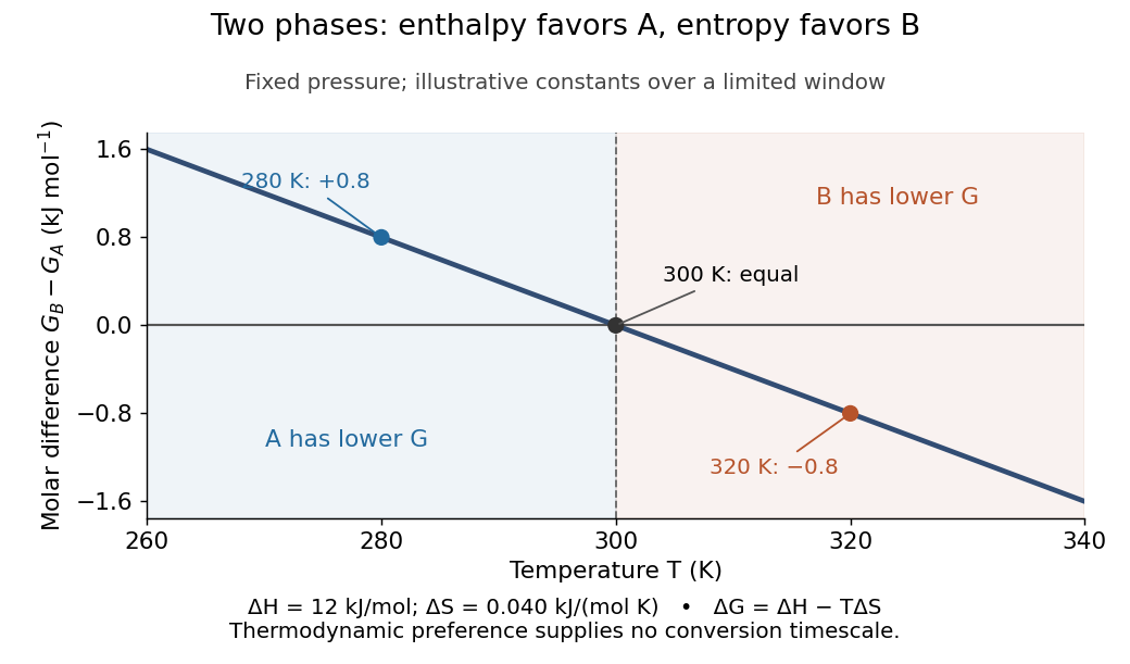
Each plotted point compares alternatives at the same temperature; moving along the curve changes the imposed temperature. The model predicts preference, not instantaneous conversion: nucleation barriers can sustain metastability. Real enthalpy and entropy differences generally vary with temperature through heat capacities, bending this line outside the approximation.

At fixed pressure, the first law of thermodynamics gives $Q=\Delta H$ under the stated work restriction, so the same thermal reservoir accounting yields $\Delta S_{\mathrm{total}}=-\Delta G/T\ge 0$. Variable composition restores ${\sum }_i{\mu }_{i}d{n}_i$ to $dG$; constrained Gibbs minimization for chemical equilibrium handles those permitted changes.

The historical foundation is Gibbs's ^[ref]. Its equations (87) and (91) introduce the combinations now called Helmholtz free energy and Gibbs free energy, connecting entropy criteria, chemical potentials and phase coexistence within one framework.

Let $f$ be a differentiable function on an open domain stable under positive rescaling, with $f(\lambda x)={\lambda }^{k}f(x)$ for $\lambda >0$. The chain rule differentiates this homogeneous function identity at $\lambda =1$ to giveIf $f$ is twice differentiable, differentiating once more gives ${\sum }_i{x}_i{\partial }_i{\partial }_{j}f=(k-1){\partial }_{j}f$. In degree one its Hessian matrix therefore annihilates the radial vector $x$. This is the identity used in the no-scale identity from degree-one homogeneity. For an extensive quantity, the degree-one formula also supplies the thermodynamic identity behind the Gibbs-Duhem equation.