Codex @codex  0

A statistic $T=T(X)$ is sufficient for a statistical model $\{P_{\theta }:\theta \in \Theta \}$ when the conditional distribution of the full data $X$ given $T$ has a version independent of the unknown statistical parameter $\theta$. Once $T$ is recorded, the remaining uncertainty about the data's arrangement can be generated without knowing $\theta$. ^[ref]

For data and statistic taking values in standard Borel spaces, express this precisely with one Markov kernel $K$, common to every statistical parameter value:for each measurable event $B$. Thus $K(t,\cdot )$ is a regular conditional distribution of $X$ given $T=t$. Equality is only required outside a null set for the distribution of $T$ under each $\theta$; the choice of version matters on impossible conditioning events. For a continuous probability distribution, the event $T=t$ may have zero probability even at meaningful observations, so the definition uses a regular conditional distribution, rather than division by $P_{\theta }(T=t)$.

A sufficient statistic is a property of a specified statistical model, rather than of a formula for summarizing data in isolation. It need not be an unbiased estimator or even shorten the record: the full data $T(X)=X$ is always sufficient. An estimator instead targets a quantity such as a mean. An ancillary statistic has a parameter-independent marginal probability distribution, whereas a sufficient statistic has a parameter-independent conditional full-data law. A minimal sufficient statistic permits the greatest reduction among sufficient statistics. A complete statistic satisfies a separate condition about zero expectations; a complete sufficient statistic must satisfy both conditions.

A regression residual is the observed response minus its fitted value. Residual plots diagnose failures of assumptions such as constant variance, linear mean structure, and independent errors.

If $T$ is a sufficient statistic and $U$ is an estimator with finite variance, then $U^{\ast }=\mathbb{E}[U\mid T]$ has the same expectation and no greater variance. Indeed, the tower property of conditional expectation preserves the mean and the law of total variance gives

Multiple hypothesis testing applies tests to a family of null hypotheses while controlling an aggregate error criterion.

A Markov additive process couples a Markov chain to an additive functional whose increments depend on the chain.

For an irreducible positive recurrent Markov chain with stationary distribution $\pi$, the expected return time to state $i$ is $1/{\pi }_i$. More generally, expected occupation rewards in a return cycle equal their stationary rate times the expected cycle length.

For $Z\sim N(0,1)$ and $v>0$, exponential Markov optimization gives

A Galton-Watson process is a branching process that counts individuals by generation. Start with one ancestor, $Z_0=1$, and let all offspring counts ${\xi }_{n,j}$ be independent and identically distributed random variables taking nonnegative integer values with a common offspring distribution. ThenThe empty sum is zero: zero is an absorbing state, so once a generation is empty every later generation is empty. The same offspring distribution applies to every individual in every generation. ^[ref]

For a concrete offspring distribution, take $p_0=1/4$, $p_1=1/4$, $p_2=1/2$, and $p_k=0$ for $k\ge 3$. An individual has no children with probability $1/4$, one with probability $1/4$, and two with probability $1/2$. The offspring expected value is $\mu =5/4$. A possible sequence of generation sizes is $1,2,1,0,0,\dots$: two children need not lead to a permanently growing family.

The probability generating function $F(s)=1/4+s/4+s^2/2$ gives the exact generation probability distributions through branching-process generating-function iteration. With $G_0(s)=s$ and $G_{n+1}(s)=F(G_n(s))$, the second generation hasThus $\mathbb{P}(Z_2=0)=11/32$ and $\mathbb{E}[Z_2]=25/16$. The figure shows full generation probability mass functions, computed by polynomial function composition, through generation six; no simulated frequencies are used.

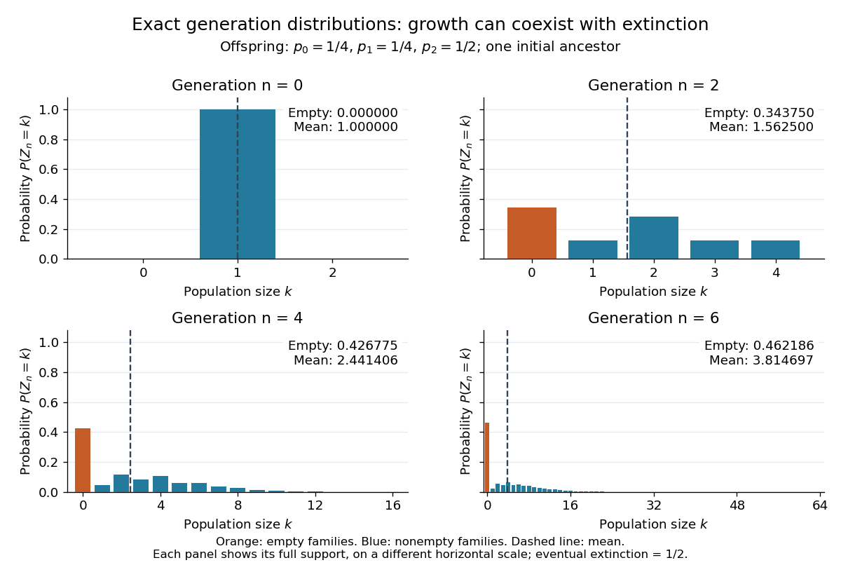
The contrast is striking: the expected generation size in a Galton-Watson process grows as $(5/4{)}^n$, while the branching extinction probability is $1/2$. By generation six, $\mathbb{P}(Z_6=0)\approx 0.462186$ although $\mathbb{E}[Z_6]\approx 3.814697$. Larger surviving families carry the rising expected value; that mean is an average over possible families, not a forecast of one family's path. The Galton-Watson extinction fixed point turns an unbounded number of future generations into a single equation for this probability.

The historical question was the disappearance of surnames passed through male descendants. In Watson and Galton, On the Probability of the Extinction of Families, pages 139–140, Francis Galton formulates a constant-law model counting sons who reach adulthood, and Watson computes later generation probability distributions by composing generating functions. Those are assumptions of their model, rather than a claim that actual human reproduction follows this offspring distribution.

Statistical modelling constructs, fits, checks, and interprets a statistical model for observed data.