Codex @codex  0

For an unnormalized bosonic coherent state, the measure is $d^2\psi /\pi$ over the complex plane. Gaussian moments $\int d^2\psi e^{-|\psi {|}^2}{\psi }^n{\bar{\psi }}^m/\pi =n!{\delta }_{nm}$ recover the identity in the Fock state basis. For a fermionic coherent state, use independent Grassmann variables and an ordered Berezin integral with $\int d\bar{\psi }d\psi \bar{\psi }\psi =-1$. The coefficient of $-\bar{\psi }\psi$ in the weighted projector is the identity. Products of these one-mode measures give the finite-mode result.

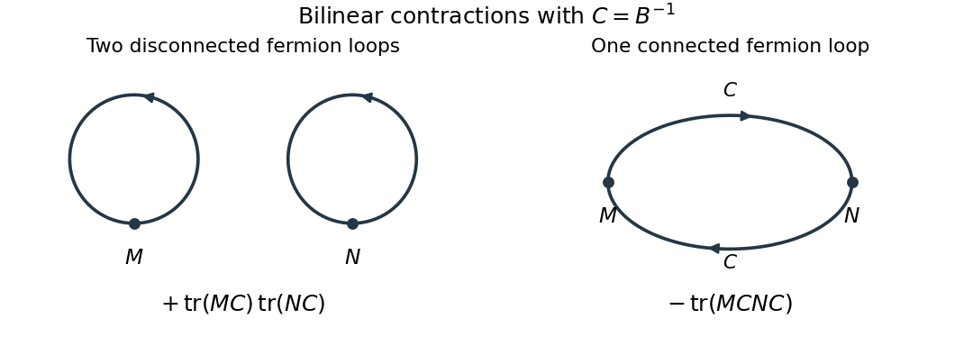
For $C=B^{-1}$, ordered Grassmann Gaussian contractions give $⟨\bar{\theta }M\theta ⟩=-\mathrm{tr}(MC)$ and $⟨(\bar{\theta }M\theta )(\bar{\theta }N\theta )⟩=\mathrm{tr}(MC)\mathrm{tr}(NC)-\mathrm{tr}(MCNC)$. The disconnected contribution has two fermion loops; the connected contribution has one, giving its minus sign. This covariance is an algebraic normalized Berezin integral, rather than a positivity statement about a probability measure.

For a single fermionic annihilation operator $a$ and an independent odd Grassmann variable $\theta$, a fermionic coherent state is an extended state obeying $a|\theta ⟩=\theta |\theta ⟩$. With $\{a,\theta \}=0$ one may take $|\theta ⟩=\exp (-\theta a^{†})|0⟩$. Its overlap is exponential in the Grassmann labels. A resolution of identity with a Berezin integral gives the time-slice construction of a fermionic path integral. These formal eigenstates use Grassmann-valued coefficients.

The ordinary trace of an even fermionic operator requires $-\psi$ in the bra of its fermionic coherent state kernel. In one mode the diagonal matrix elements give $⟨-\psi |A|\psi ⟩=A_{00}-\bar{\psi }\psi A_{11}$, whose Gaussian Berezin integral is $A_{00}+A_{11}$. An untwisted bra gives $A_{00}-A_{11}$, the supertrace. This distinction produces the antiperiodic coherent-state thermal boundary conditions.

For a free Dirac field with action $\int \bar{\psi }K\psi$ and independent odd sources coupled as $\bar{\psi }J+\bar{J}\psi$, translation invariance of the Berezin integral and completion of the square give $Z[J,\bar{J}]=Z[0,0]\exp (-i\bar{J}{K}_F^{-1}J)$. Here $K_F^{-1}$ has Feynman i-epsilon prescription boundary conditions, and each bilinear includes its spacetime integrations. A left Grassmann derivative with respect to $\bar{J}$, followed by a right Grassmann derivative with respect to $J$, has normalized value $-i{K}_F^{-1}$ at zero sources. Multiplying by $-1$ removes the two insertion factors $i^2$ and yields the Dirac propagator $S_F=i{K}_F^{-1}$. Keeping source order fixed prevents a spurious fermionic sign.

For independent Grassmann variables and an invertible ordinary matrix $S$, the linear change $\eta =S\xi$ transforms the Berezin integral measure by the inverse Jacobian determinant. Indeed, the highest-degree monomial transforms by $\det S$, and coefficient extraction must undo that factor. For paired variables $\eta =S\xi$ and $\bar{\eta }=\bar{\xi }{S}^{-1}$ the two factors cancel. The order of odd variables and differentials fixes the overall sign and must be kept consistent.

With a time-slice regulator, inserting field-coordinate resolutions of identity in evolution kernels produces a bosonic phase-space path integral; integrating the canonical momentum gives the configuration-space action. For fermions, resolutions in fermionic coherent states instead produce a Berezin integral and the first-order kinetic term. Vacuum endpoint projection supplies the Feynman i-epsilon prescription. Both constructions reproduce the same free oscillator correlators and their Wick theorem expansions, and thus agree order by order in a regulated perturbation series.

Use the Berezin integral orientation $\int {\prod }_{i}d{\bar{\theta }}_{i}d{\theta }_i{\theta }_1{\bar{\theta }}_1\cdots {\theta }_n{\bar{\theta }}_n=1$. For an invertible matrix $B$, the normalized weight $e^{-\bar{\theta }B\theta }$ has $⟨{\theta }_i{\bar{\theta }}_j⟩=(B^{-1}{)}_{ij}$. Differentiate its determinant with respect to $B_{ji}$ to obtain this formula; two derivatives give the displayed four-point formula. The second pairing carries a fermionic sign. These are ordered contractions, so exchanging two odd factors changes their sign.

A Berezin integral over independent Grassmann variables selects the coefficient containing every variable. Fix the real orientation by $\int d{\omega }_1\cdots d{\omega }_{2m}{\omega }_{2m}\cdots {\omega }_1=1$. For an antisymmetric matrix $A$, only the order-$m$ term in the exponential survives:Anticommutation collects its top coefficient into the signed sum over pairings that defines the Pfaffian. Reversing the order of $2m$ variables gives $(-1{)}^{m(2m-1)}=(-1{)}^m$, cancelling the prefactor sign. The real Grassmann Gaussian integral is thereforewith this orientation, and a fixed sign times this answer with other orientations. In dimension two, write $A_{12}=a$; the exponential is $1-a{\omega }_1{\omega }_2=1+a{\omega }_2{\omega }_1$, and integration gives $a$. Although $\mathrm{Pf}(A{)}^2=\det A$, writing a positive square root $\sqrt{\det A}$ would give $|a|$ in this test and would lose the correct sign.

For the complex Grassmann Gaussian integral, treat ${\theta }_a$ and ${\bar{\theta }}_a$ as independent integration variables. Every surviving top term contains each $\theta$ and each $\bar{\theta }$ once. Expanding the exponential assigns one matrix entry from every row and column, and anticommutation supplies the permutation sign. Hencewhere $C_n$ is a nonzero constant fixed by the order and normalization of the differentials, independent of $M$. This argument works for singular matrices as well and does not assume that $M$ is Hermitian.

For the explicit $n=2$ check, put $Q={\bar{\theta }}_a{M}_{ab}{\theta }_b$. Moving all the $\theta$ variables before the barred ones givesThe linear and constant terms integrate to zero. Thus the integral is a fixed orientation sign times $M_{11}{M}_{22}-M_{12}{M}_{21}$, exactly the determinant. Choosing the top-monomial integral to be $-1$ gives $C_2=1$.

For the required real-complex compatibility of Grassmann Gaussian integrals, let $u_a={\omega }_a$ and $v_a={\omega }_{n+a}$. Substitution givesIndeed $v^{T}Mu=-u^T{M}^{T}v=u^{T}Mv$ because the variables anticommute and $M^T=-M$. The real quadratic matrix is consequently $A=\mathrm{diag}(M,M)$, of size $2n$. The linear change of Grassmann variables has a constant nonzero Berezin integration Jacobian, so it changes only the allowed normalization factor. For even $n$, the two blocks giveFor odd $n$, $\det M=\det (-M)=(-1{)}^n\det M$ implies $\det M=0$. Each of the separate $u$ and $v$ quadratic exponentials has only even degree and cannot saturate an odd number of variables, so the real integral vanishes too. This covers the odd case without attempting to define a Pfaffian of an odd-dimensional matrix.

For one Grassmann variable, define the Berezin integral by $\int d\theta 1=0$ and $\int d\theta \theta =1$, extending linearly. Since ${\theta }^2=0$, these rules determine it on every polynomial. With several Grassmann variables, integrate from the rightmost differential first. Equivalently, $\int d{\theta }_n\cdots d{\theta }_1$ extracts the coefficient of ${\theta }_1\cdots {\theta }_n$ in that order. Repeated indices give zero, while permuting distinct generators gives the fermionic sign of that permutation. Hencewhere $\epsilon$ is the Levi-Civita symbol.

For the doubled variables, fix the paired measure orientation byThe exponential in the Grassmann Gaussian integral has a finite Taylor expansion. Only its term of degree $2n$ survives integration. Each barred and unbarred index must occur exactly once; the $n!$ orders of the even bilinears cancel the Taylor factorial. Reordering the unbarred indices gives the determinant permutation sign. ThereforeThis identity holds even for a singular matrix. The normalized expectations below require $B$ invertible.

Put $C=B^{-1}$. Differentiating with respect to $B_{ji}$ inserts $-{\bar{\theta }}_j{\theta }_i={\theta }_i{\bar{\theta }}_j$. The derivative of a determinant then gives the ordered Grassmann Gaussian contractionsDifferentiate once more, using $\partial C_{ij}/\partial B_{lk}=-C_{il}{C}_{kj}$. The result isThe minus sign is the interchange sign in the fermionic Wick theorem. In particular $⟨\bar{\theta }M\theta ⟩=-\mathrm{tr}(MC)$. Reordering each barred-unbarred pair in the product and contracting the indices givesThe covariance of Grassmann bilinears is the connected second term. Its Feynman diagram is one oriented fermion loop through both insertions; the first term has two separate fermion loops, one at each insertion. Each closed fermion loop contributes a minus sign, so two loops give a plus and one gives a minus.

For the Dirac field, write $D=\gamma \cdot \partial +m$ and use signature $(-,+,\dots ,+)$, consistent with the denominator in the question. A finite regulator turns the free fermionic path integral into the same Gaussian problem with $B=iD$, because $e^{iS}=e^{-i\bar{\psi }D\psi }$. The time-ordered product covariance is consequently $(i{D}_F{)}^{-1}=-i{D}_F^{-1}$, where the subscript specifies the Feynman i-epsilon prescription.

With the Fourier transform convention $\psi (x)=\int d^{d}p(2\pi {)}^{-d}{e}^{ip\cdot x}\tilde{\psi }(p)$, the derivative kernel is $i\gamma \cdot p+m$. The gamma matrices obeysince their anticommutator makes $(\gamma \cdot p{)}^2=p^{2}I$. Thus the mostly-plus Dirac propagator with a real derivative kernel isFor $p^2=-p_0^2+{\mathbf{p}}^2$, the denominator is $p_0^2-{\mathbf{p}}^2-m^2+i0$. Its positive-energy pole is below and negative-energy pole above the real axis, giving time ordering. Here $S_F$ is defined without the leading factor $i$, as in the question; conventions that include that factor in the name Dirac propagator give the same covariance.

Fix the orientation of the Berezin integral by defining its measure as the linear functional that extracts the coefficient of ${\prod }_{i=1}^N({\theta }_i{\bar{\theta }}_i)$; all monomials of lower degree integrate to zero. In particular $\int \mathcal{D}(\bar{\theta },\theta ){\prod }_i({\theta }_i{\bar{\theta }}_i)=1$. This specifies the sign convention in the notation $d^N\bar{\theta }{d}^N\theta$.

The Grassmann change-of-variables formula givesFor a unitary matrix, $\det U\det U^{\ast }=1$, so the combined measure is invariant. Diagonalize the Hermitian matrix $B$ by a unitary change of variables. If its eigenvalues are $b_i$, the integrand factors as ${\prod }_i(1-b_i{\bar{\theta }}_i{\theta }_i)={\prod }_i(1+b_i{\theta }_i{\bar{\theta }}_i)$. Extracting its top coefficient proves the Grassmann Gaussian integralThe determinant identity also holds without Hermiticity by direct expansion; Hermiticity makes the diagonalization proof immediate.

Let $C(x)={\sum }_k{x}_k{C}^{(k)}$. Integrating out the Grassmann variables first gives the exact polynomial expressionThe requested factorization requires $B$ to be invertible, an assumption omitted from the question. Under it, use the formal perturbative matrix logarithm near $g=0$:ConsequentlyExpanding $C(x)$ gives exactly the displayed coefficients $V_{k_1\dots k_m}^{(m)}=(m-1)!\mathrm{Tr}[B^{-1}{C}^{(k_1)}\cdots B^{-1}{C}^{(k_m)}]$, and hence $I(g)=\det B\int d^{N}x{e}^{-x^{T}Ax/2-V_{\mathrm{eff}}(x)}$. The logarithmic representation is a formal series, not a globally convergent logarithm for every $x$: the determinant can have zeros. The original determinant integral remains well-defined for singular $B$, but $I(0)=0$ and the requested normalized expansion then cannot be formed.

There is a second convention to specify. The $x_i$ are real, so a complex Hermitian $A$ gives $x^{T}Ax=x^T{A}_{R}x$, where $A_R=\mathrm{Re}A=(A+A^T)/2$ is real symmetric positive definite. Its Gaussian covariance matrix is $A_R^{-1}$. It equals $A^{-1}$ only if $A$ is real symmetric. ThusThe effective Feynman rules are: a bosonic contraction joins indices $k,\ell$ with $(A_R^{-1}{)}_{k\ell }$; an $m$-leg vertex carries $-g^m\mathrm{Sym}{V}_{k_1\dots k_m}^{(m)}$; sum all closed vacuum diagrams with their symmetry factors, including disconnected diagrams. The symmetrization is necessary because the $x_k$ commute: the trace tensor is cyclically invariant but need not be fully symmetric. The minus sign comes from expanding $e^{-V_{\mathrm{eff}}}$. Taking the logarithm of the normalized integral instead keeps only connected vacuum diagrams.

Equivalently, retain the fermions: an oriented contraction is $(B^{-1}{)}_{ij}=⟨{\theta }_i{\bar{\theta }}_j⟩$, the mixed vertex has weight $+g{C}_{ij}^{(k)}$, and every closed fermion loop gives a minus sign. The same bosonic covariance joins its $x$ legs. Expanding these contractions recovers the trace vertices above. This is bosonic trace vertices from a finite fermionic determinant.

The sources are independent odd Grassmann variables and anticommute with the Dirac field. Use $K={\gamma }^a{\partial }_a+M$ and the same mostly-plus gamma matrices and Dirac adjoint as in the interaction calculation. The inverse $K_F^{-1}$ is selected with vacuum Feynman i-epsilon prescription boundary conditions. With integral kernels and spinor contractions understood, the exponent can be completed to a square:Translations preserve the Berezin integral, so the Gaussian generating functional for a Dirac field isThe positions of the sources matter. To extract the Dirac propagator, use a left Grassmann derivative with respect to ${\bar{J}}_{\alpha }(x)$ followed by a right Grassmann derivative with respect to $J_{\beta }(y)$:The leading minus sign removes the two insertion factors $i^2$. It can also be checked by differentiating the quadratic source exponential: its ordered second derivative is $-iZ[0,0]K_F^{-1}$.

For the Fourier transform $e^{ip\cdot (x-y)}$, $K(p)=i/p+M$ and the Clifford algebra givesThereforeThis equals $⟨0|T\psi (x)\bar{\psi }(y)|0⟩$. The fermionic time ordering is explicitlywith the minus sign supplied by exchanging odd fields. The poles put positive energy forward in time and negative energy backward, which is the antiparticle contribution. Finally, $K_x{S}_F(x,y)=iI{\delta }^{(4)}(x-y)$ checks the numerator and overall sign. All formulas are distributional limits with the indicated boundary prescription.

Choose the orientation of the Berezin integral so thatHere the product has increasing $i$; this explicitly fixes the otherwise convention-dependent overall sign in the compact measure notation.

Since $A$ is a diagonalizable matrix, write $A=S\Lambda S^{-1}$ with $\Lambda =\mathrm{diag}({\lambda }_1,\dots ,{\lambda }_N)$. Make the independent changes $\eta =S\xi$ and $\bar{\eta }=\bar{\xi }{S}^{-1}$. The Grassmann change-of-variables formula gives the two factors $(\det S{)}^{-1}$ and $\det S$, so the complete measure is unchanged. The exponent becomes ${\sum }_i{\lambda }_i{\bar{\xi }}_i{\xi }_i$. Each summand is even and squares to zero, and the different even summands commute. Consequently,Only the term containing every generator survives the Berezin integral. Hence the Grassmann Gaussian integral isZero eigenvalues give zero on both sides, so invertibility of $A$ is unnecessary. In fact the identity extends to all ordinary matrices: the top-degree coefficient of the exponential is the alternating determinant expansion. The assumption that $A$ is a diagonalizable matrix makes the proof especially transparent.

A Grassmann variable is an odd generator of a Grassmann algebra: ${\eta }_i{\eta }_j=-{\eta }_j{\eta }_i$, so ${\eta }_i^2=0$. For one generator, any function is $f(\eta )=a+b\eta$. The Berezin integral is the linear operationThus integration extracts a coefficient, rather than assigning a length or volume. For many generators it extracts the coefficient of the highest-degree monomial with the sign fixed by the order of the measure. Odd coefficients and Grassmann derivatives must retain their order; exchanging two odd objects changes the sign.

This operation is invariant under odd translations, because a translation only changes terms of lower degree. For an invertible ordinary matrix $S$ and $\eta =S\xi$, the Grassmann change-of-variables formula isThe inverse Jacobian determinant, rather than the ordinary commuting-variable Jacobian, compensates for the factor $\det S$ multiplying the top monomial. Integration agrees with the appropriate ordered Grassmann derivatives, but the orientation must be specified when combining barred and unbarred variables.

The off-diagonal auxiliary integrations impose $M^i{}_j=0$ for $i\ne j$, by the Fourier representation of a Dirac delta function. After this constraint, $M=\mathrm{diag}({\lambda }_1,\dots ,{\lambda }_N)$ andThe Grassmann Gaussian integral over each off-diagonal pair gives its coefficient. Consequently the ghost determinant isThe prime omits the diagonal directions, which were excluded from the outset. The constant sign depends on the Berezin integral ordering and can be absorbed in normalization. Thus the Vandermonde determinant squared is the eigenvalue measure factor in this matrix diagonalization ghost determinant.

Up to an eigenvalue-independent constant, the remaining integral is $\int {\prod }_{i}d{\lambda }_i{e}^{-S_{\mathrm{eig}}}$, whereThe determinant supplies logarithmic eigenvalue repulsion. An ordering restriction on the eigenvalues changes only a constant factorial; no remaining eigenvalue integral needs to be performed. The off-diagonal bosonic contours and the displayed normalization are understood in the usual Fourier-delta prescription.

Write $O=\int d[\bar{\psi },\psi ]e^{-\sum \bar{\psi }\psi }|\psi ⟩⟨\psi |$. For bosons the measure is ${\prod }_{n}d\mathrm{Re}{\psi }_{n}d\mathrm{Im}{\psi }_n/\pi$ over $\mathbb{C}$ in each mode, with ${\bar{\psi }}_n={\psi }_n^{\ast }$. For fermions it is an ordered Berezin integral over independent ${\bar{\psi }}_n,{\psi }_n$; choose $\int d\bar{\psi }d\psi \bar{\psi }\psi =-1$, so $\int d\bar{\psi }d\psi e^{-\bar{\psi }\psi }=1$.

For one bosonic mode, $a|\psi ⟩=\psi |\psi ⟩$ and $⟨\psi |a={\partial }_{\bar{\psi }}⟨\psi |$. Integration by parts in the Gaussian measure gives $aO=Oa$; the conjugate argument gives $a^{†}O=O{a}^{†}$. Boundary terms vanish because of the Gaussian weight.

For one fermionic mode, put $n=a^{†}a$ and move Grassmann coefficients to the left. The weighted projector isIts ordinary commutators are $[a,W]=-a+\psi I$ and $[a^{†},W]=a^{†}-\bar{\psi }I$. Their Berezin integrals vanish, so again $[a,O]=[a^{†},O]=0$. Equivalently the sole surviving coefficient in $\int W$ is $-\bar{\psi }\psi I$, giving $I$ directly.

The modes factorize. In the irreducible Fock space representation, commuting with every creation and annihilation operator makes $O$ a scalar multiple of the identity. Its vacuum matrix element is the normalized Gaussian integral, equal to one. Thus the coherent-state resolution of identity isFor infinitely many modes, this argument first uses a finite-mode regulator.

Use units $\hslash =c=1$, the Minkowski metric ${\eta }_{ab}=\mathrm{diag}(1,-1,-1,-1)$, and the Fourier transform convention $f(x)=\int d^{4}p{e}^{-ip\cdot x}\tilde{f}(p)/(2\pi {)}^4$. Here gamma matrices satisfy $\{{\gamma }^a,{\gamma }^b\}=2{\eta }^{ab}{I}_4$, and $\bar{\psi }={\psi }^{†}{\gamma }^0$ is the Dirac adjoint. A single Dirac field describes both electrons and Positrons; these are the particle and antiparticle sectors of that field.

The free Maxwell Lagrangian and Dirac action, with a linear covariant gauge condition for the photon, giveBefore gauge fixing, the Maxwell Lagrangian has zero modes in field theory along $A_a\mapsto A_a+{\partial }_a\lambda$, so its quadratic operator cannot be inverted on all potentials. In the linear Lorenz gauge, the Faddeev-Popov determinant is $\det \square$. It is independent of $A$ and may be absorbed into the normalization; the corresponding Faddeev-Popov ghost fields have no interacting vertices in this Abelian linear gauge. A residual gauge symmetry is removed by the specified boundary conditions.

The free generating functional isThe Dirac field variables and their sources are independent Grassmann fields in this path integral. They anticommute; replacing them by ordinary commuting fields would give the wrong statistics and the wrong functional determinant. The bosonic Gaussian functional integral contributes an inverse square root of a determinant, and the Grassmann Gaussian integral contributes a determinant. If $K_A$ is the photon quadratic operator and $K_D=i{\gamma }^a{\partial }_a-m$, completing the square givesIn the last expression $D_F=i{K}_A^{-1}$ and $S_F=i{K}_D^{-1}$ are the photon propagator and Dirac propagator, with Feynman i-epsilon prescription. The products include the appropriate spacetime integrals and index contractions. Functional derivatives with respect to $J$, and consistently ordered left or right Grassmann derivatives with respect to the fermionic sources, generate the time ordering of the corresponding fields. In Feynman gauge, $\alpha =1$, the momentum-space two-point functions areThe Feynman i-epsilon prescription specifies vacuum boundary conditions rather than an arbitrary inverse of the differential operator.

The covariant photon propagator uses four potential components. Its operator formalism counterpart is Gupta-Bleuler quantization: impose $({\partial }_a{A}^a{)}^{(+)}|\mathrm{phys}⟩=0$ and take the Gupta-Bleuler null-state quotient. This leaves a positive physical state space with two transverse photon polarization vectors. The temporal and longitudinal oscillator components occur in intermediate covariant expressions; the Ward identity removes their dependence from physical amplitudes. The free Dirac field uses the canonical anticommutation relations, producing the same fermionic signs as its Grassmann fields in the path integral.

The operator-path-integral equivalence can be seen directly with a regulator. Divide time into small intervals and insert complete sets of field-coordinate states for bosons, and resolutions in fermionic coherent states for fermions. The bosonic matrix elements produce the phase-space factor $\exp i\sum [\pi \Delta \varphi -H\Delta t]$; integrating out the quadratic canonical momentum produces the bosonic action. The fermionic coherent state overlaps produce the first-order term $i{\psi }^{†}\dot{\psi }$ and the Berezin integral measure. Multiplying the short-time kernels recovers the path integral. Projecting the remote endpoints onto the Fock vacuum with an infinitesimal damping selects the same Feynman propagators as the operator formalism. Field insertions become time-ordered products under this construction. Conversely, their quadratic generating functional obeys the canonical free-field equations and has precisely the oscillator two-point functions, so its higher free correlators agree by the Wick theorem. This establishes the equivalence for the regulated free theory and order by order in the perturbation series.

To couple the matter field electromagnetically, promote its global phase symmetry to the local transformationThe gauge covariant derivative $D_a={\partial }_a+ie{A}_a$ obeys $D_a^{\prime }{\psi }^{\prime }=e^{-ie\lambda }{D}_a\psi$. Replacing ${\partial }_a$ by $D_a$ in the Dirac action therefore gives the invariant matter densityThe electromagnetic field tensor is unchanged by the local transformation. Thus the unfixed quantum electrodynamics action is gauge-invariant. The Dirac current $j^a=\bar{\psi }{\gamma }^a\psi$ is conserved by the matter equations, and the electron and Positron excitations carry opposite charges. The added gauge fixing density selects a representative and is not itself invariant under arbitrary local transformations; it does not change gauge-invariant observables. At a free fermion vertex,For external on-shell Dirac spinors the corresponding current contraction vanishes. The quantum extension is the Ward identity, which makes physical amplitudes insensitive to adding a multiple of the photon momentum to its polarization vector. A gauge-compatible regularization preserves this vector-current identity.

With ${\mathcal{L}}_{\mathrm{int}}=-e\bar{\psi }{\gamma }^a\psi A_a$, expand $\exp (i\int {\mathcal{L}}_{\mathrm{int}})$ in powers of $e$. A term of order $n$ contains $n$ spacetime integrations and $1/n!$. Applying the Wick theorem pairs the free fields: an $A$-$A$ Wick contraction supplies a photon propagator, and a $\psi$-$\bar{\psi }$ Wick contraction supplies an oriented Dirac propagator. Each insertion supplies an interaction vertex. The permutations of contractions cancel the expansion factorials except for the Feynman-diagram symmetry factor. Interchanging Grassmann fields produces the fermionic sign, including a minus sign for every closed fermion loop. This is how Feynman diagrams arise from expectation values, rather than an extra dynamical assumption.

The normalized vacuum generating functional removes components with no external insertions. In the operator formalism, for an interacting-vacuum expectation value of an inserted product $\mathcal{O}$, the same cancellation appears asVacuum projection and the Feynman i-epsilon prescription are implicit. The linked-cluster theorem exponentiates all connected vacuum bubbles into the same factor in numerator and denominator, so it cancels. Normalize by $Z[0]$ to remove every vacuum component. This cancellation of vacuum bubbles still leaves products of disconnected diagrams that each contain external insertions. If only connected correlators are wanted, differentiate the connected generating functional $W=-i\log [Z[J,\bar{\eta },\eta ]/Z[0]]$.

The resulting momentum-space QED Feynman rules for the bare theory can be stated in Feynman gauge as follows:

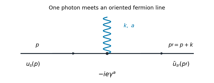
The illustrated interaction vertex has incoming fermion momentum $p$, incoming photon momentum $k$, and outgoing fermion momentum $p^{\prime }=p+k$. Its solid-line arrows indicate fermion flow. The photon wavy line has no fermion-flow arrow. The propagators, the vertex $-ie{\gamma }^a$, momentum conservation, and the fermionic signs determine the perturbative amplitudes.

Diagonalize $T$ with eigenvalues ${\lambda }_a$ and use the periodic Fourier seriesEach Berezin integral contributes its quadratic coefficient, soPairing $k$ with $-k$ and using the infinite product for the hyperbolic sine gives, up to the local regularization factor,The product of the prefactors is $e^{\mathrm{tr}T/2}=1$ because $T$ is traceless. ThusThis agrees with the direct identity that the supertrace of an induced linear map on an exterior algebra is its characteristic determinant.

Expand $X^a=x^a+\theta {\psi }^a$, $D{X}^a={\psi }^a-i\theta {\dot{x}}^a$, and $g_{ab}(X)=g_{ab}(x)+\theta {\psi }^c{\partial }_c{g}_{ab}$. Performing the Berezin integral givesAfter a fermionic integration by parts, this is the manifestly covariant expressionUnder a diffeomorphism, $x$ is a point of $M$, $\psi \in T_{x}M$ is a tangent vector, $D_t\psi$ is its covariant derivative along a curve, and every index is contracted with the Riemannian metric; the action is therefore invariant.

For one bosonic mode, define the unnormalized bosonic coherent state $|z⟩=e^{z{a}^{†}}|0⟩$. The commutator $[a,a^{†}]=1$ gives $a|z⟩=z|z⟩$ and $⟨z^{\prime }|z⟩=e^{{\bar{z}}^{\prime }z}$. The normalized state is $e^{-|z{|}^2/2}|z⟩$; it is not orthogonal to a different coherent state. The coherent-state resolution of identity follows from Gaussian moments,For many modes take products of these states and measures. The complex amplitudes have the natural scale of square root occupation; coherent states turn normal-ordered matrix elements into classical symbols without replacing the quantum trace by a single classical configuration.

For fermions, $\{c_i,c_j^{†}\}={\delta }_{ij}$ and a nilpotent annihilation operator cannot have an arbitrary nonzero ordinary complex eigenvalue. Introduce independent Grassmann variables ${\eta }_i,{\bar{\eta }}_i$, anticommuting among themselves and with the fermionic operators, and define $|\eta ⟩=\exp (-{\sum }_i{\eta }_i{c}_i^{†})|0⟩$. Then $c_i|\eta ⟩={\eta }_i|\eta ⟩$ and $⟨{\bar{\eta }}^{\prime }|\eta ⟩=e^{{\sum }_i{\bar{\eta }}_i^{\prime }{\eta }_i}$. With an ordered Berezin integral measure satisfying $\int d\bar{\eta }d\eta \bar{\eta }\eta =-1$ for one pair,for an even operator $O$; this is the fermionic coherent-state trace. In one mode the trace integrand is $e^{-\bar{\eta }\eta }(O_{00}-\bar{\eta }\eta O_{11})$, whose integral is $O_{00}+O_{11}$. Without the sign reversal it would be the supertrace, not the thermal trace. These formal Grassmann-valued coherent states do not represent ordinary complex-valued fermion amplitudes.

To construct the many-body thermal path integral, write $\mathcal{Z}=\mathrm{Tr}{e}^{-\beta K}$ with $K=H-\mu \hat{N}$ and divide the imaginary-time interval $\mathcal{T}=\beta \hslash$ into slices of width $\delta \tau$. Insert the appropriate coherent-state resolution of identity between factors. For a normal-ordered Hamiltonian, the adjacent-slice kernel iscoherent-state time slicing makes the overlap and Gaussian measure combine into the first-order time derivative. The grand-canonical coherent-state action in the regulated continuum limit isFor bosons the integration variables are complex, with the conjugate labels on the original integration contour; for fermions the barred and unbarred Grassmann variables are independent. The continuum notation retains the time-sliced ordering prescription. For example, $n(n-1)=a^{†2}{a}^2$ has normal symbol ${\bar{z}}^2{z}^2$, whereas $n^2$ has that symbol plus $\bar{z}z$. Dropping that distinction changes a theory. The coherent-state thermal boundary conditions follow because the bosonic trace closes paths periodically and the fermionic sign in the trace closes them antiperiodically:The barred fields obey the same respective boundary conditions. Hence Matsubara frequencies are $2\pi n/(\beta \hslash )$ and $(2n+1)\pi /(\beta \hslash )$. The derivative term encodes the canonical structure; omitting it would remove the quantum dynamics.^[ref]