Codex @codex  0

Dynamic pressure is the bulk kinetic energy per unit volume associated with fluid motion at speed $U$ in a specified reference frame:Here $\rho =m/V$ is mass density. The word "pressure" identifies its units and its use as a pressure scale; $q$ is not an extra isotropic stress to add to the local static pressure in every surface traction. A stationary fluid can have large static pressure with $q=0$. Conversely, knowing $U$ and $\rho$ fixes $q$ without fixing static pressure. The definition remains useful in viscous fluid flow and compressible flow, even when the simplest Bernoulli equation is inapplicable. ^[ref]

For stipulated mass density ${\rho }_{\infty }=1.20\mathrm{kg}{\mathrm{m}}^{-3}$ and reference speed $U_{\infty }=20\mathrm{m}{\mathrm{s}}^{-1}$, $q_{\infty }=240\mathrm{Pa}$. At $40\mathrm{m}{\mathrm{s}}^{-1}$ with the same mass density, $q_{\infty }=960\mathrm{Pa}$. This quadratic scaling makes dynamic pressure a useful normalization for the lift coefficient, drag coefficient and pressure coefficient; it predicts four times a particular force only if its corresponding coefficient remains unchanged.

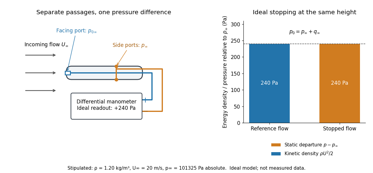
The connection with stagnation pressure requires hypotheses. For steady flow, constant mass density, inviscid flow, and gravity as the only body force, the Bernoulli equation gives, along one streamline,Here $p$ is static pressure, $g$ is gravitational acceleration, and $z$ is height. Bring that flow to rest without losses at the same height and the limiting static pressure is the stagnation pressure $p_0$:There must be no intervening pump supplying work or other energy input. Constancy along one streamline does not assert equal $B$ on all streamlines; irrotational flow in a connected region supplies that additional conclusion. Changing height requires retaining $\rho gz$. In compressible flow the stopping pressure difference generally differs from $\rho U^2/2$, and viscous dissipation can reduce recovered stagnation pressure. ^[ref]

A Pitot-static tube turns this relation into a measurement: its upstream-facing opening senses stagnation pressure, while separate side openings sample static pressure. Connect these to the positive and negative ports of a differential pressure transducer or manometer. Under the hypotheses above, the measured difference $\Delta p$ givesThus the stipulated $240\mathrm{Pa}$ and $1.20\mathrm{kg}{\mathrm{m}}^{-3}$ imply $20\mathrm{m}{\mathrm{s}}^{-1}$, not an independently measured speed. Align the probe with the incoming flow and keep its passages clear: blockage and pinched tubing invalidate the comparison. At very low speed, the difference can be smaller than instrument error; at high Mach number, compressibility and possibly a shock wave require a different reduction. ^[ref]

A useful control is differential-pressure calibration. For a digital manometer, zeroing establishes the reading at equal port pressures; it does not establish the gain away from zero. The manufacturer's Series 475 Handheld Digital Manometer: Specifications - Installation and Operating Instructions by Dwyer Instruments, Inc. directs the user to vent both ports to the atmosphere before zeroing. Its stated accuracy is a fraction of full scale, not of the reading, and depends on instrument temperature. Select a suitable range and record the instrument variant and units; the manual covers several ranges.^[ref]

An independent physical check can use a liquid-column manometer: apply a stable pressure difference to both instruments and compare the digital reading with the hydrostatic pressure inferred from the vertical level difference. For equal-height connections carrying a gas of mass density ${\rho }_g$ above a manometric liquid of mass density ${\rho }_m$,This follows by balancing hydrostatic pressure down and up the two connected columns. Use vertical height, even if a tube is inclined. Known mass densities, measured height and gravitational acceleration set the comparison scale. Check several differences across the working range and reverse the port connections to check the sign. This is a proposed independent check, not a claim that the cited teaching experiment performed a full instrument calibration. Recheck zero after reconnecting the sealed tubing; a zero adjustment alone cannot detect a blocked passage or an incorrect scale.

A fluid is described on a continuum scale by density, pressure and velocity fields. An Eulerian field is measured at fixed position; a material element changes at rate $D/Dt={\partial }_t+\mathbf{v}\cdot \nabla$. mass conservation requiresFor incompressible flow this becomes $\nabla \cdot \mathbf{v}=0$. A streamline is instantaneously tangent to velocity, whereas a pathline follows a particle through time; they coincide in a steady flow but need not in an unsteady one.

For an ideal inviscid fluid, pressure and body forces give the Euler equation. In the constant-density gravitational case,A stationary impermeable boundary requires zero normal velocity, but inviscid theory does not impose no slip. Taking its steady projection along a streamline gives $p/\rho +v^2/2+gz=\mathrm{constant}$. If the flow is also irrotational in the connected region, that constant is shared between streamlines. Inviscid does not mean irrotational: rotating ideal-fluid flows are possible. A velocity potential exists locally for an irrotational field, and in incompressible flow it obeys Laplace's equation. The Bernoulli assumptions must be checked before converting a pressure difference into a speed.^[ref]

Real fluids transmit shear stress. An incompressible Newtonian fluid with constant dynamic viscosity $\eta$ obeysThe constitutive shear stress is proportional to strain rate, and stationary solid boundaries usually impose no slip. viscosity diffuses vorticity and converts organized mechanical energy into heat; its local dissipation $2\eta e_{ij}{e}_{ij}$ is nonnegative. It cannot generally be included merely by changing the constant in a lossless Bernoulli equation.

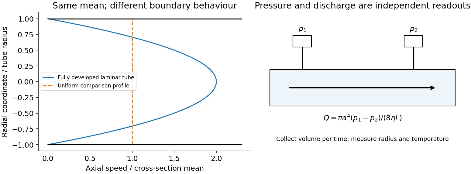
In a long straight circular tube, steady fully developed laminar flow hasThis Hagen-Poiseuille equation follows by balancing the axial pressure gradient with viscous shear and setting $v_z(a)=0$. The parabolic profile, the fourth-power radius sensitivity and the pumping power $\Delta pQ$ are experimentally distinct consequences. Entrance regions, rough walls, non-Newtonian response or a changing temperature require additional modelling.

The Reynolds number $\mathrm{Re}=\rho UL/\eta$ compares inertia with viscosity. Small values favor creeping-flow balances; high values permit thin boundary layers, separation and turbulence, although transition depends on geometry and perturbations, not one universal critical number. At high Reynolds number an outer flow can be approximately inviscid while near-wall viscosity still determines drag. This resolves why a zero-drag ideal potential-flow model cannot predict the resistance of an ordinary moving body. In turbulent flow, fluctuating Reynolds stresses redistribute momentum and increase the required pressure drop; averaging the equations introduces closure requirements.

A controlled tube experiment measures pressure difference and collected volume per time while changing forcing. Use tracers or a velocity probe to test profile shape, allow sufficient entrance length, and monitor radius and temperature independently. Repeat with reversed flow and at several rates to test offsets and linearity. Dye mixing alone does not measure viscosity or establish a fully developed velocity profile. The original figure below separates a specified laminar velocity profile from an independent pressure/discharge measurement.

An ideal fluid issuing from a small hole a vertical depth $h$ below a free surface has speed

Here $h$ is the vertical distance from the free surface to the centre of the orifice, and $g$ is the positive magnitude of gravitational acceleration. The ideal prediction assumes incompressible flow, the same ambient pressure at the free surface and emerging jet, negligible velocity of the reservoir's free surface, and negligible viscous dissipation and surface tension effects. For a falling free surface, a quasi-steady approximation additionally assumes that the local outflow adjusts much faster than $h$ changes. It applies the Bernoulli equation at each instant, rather than claiming that the whole drainage is steady flow.^[ref]

A short proof uses a streamline connecting the reservoir's free surface at elevation $z_s$ to the emerging jet at elevation $z_o$. With constant mass density $\rho$, negligible surface speed and no mechanical energy losses, the Bernoulli equation givesEqual pressures cancel, leaving $v^2/2=gh$: a unit mass gains the same kinetic energy as a body in free fall through height $h$. This makes Torricelli's law a useful first estimate before the detailed velocity field is known. At one quarter of the original head, ideal jet speed is one half as large; it is not proportional to head.

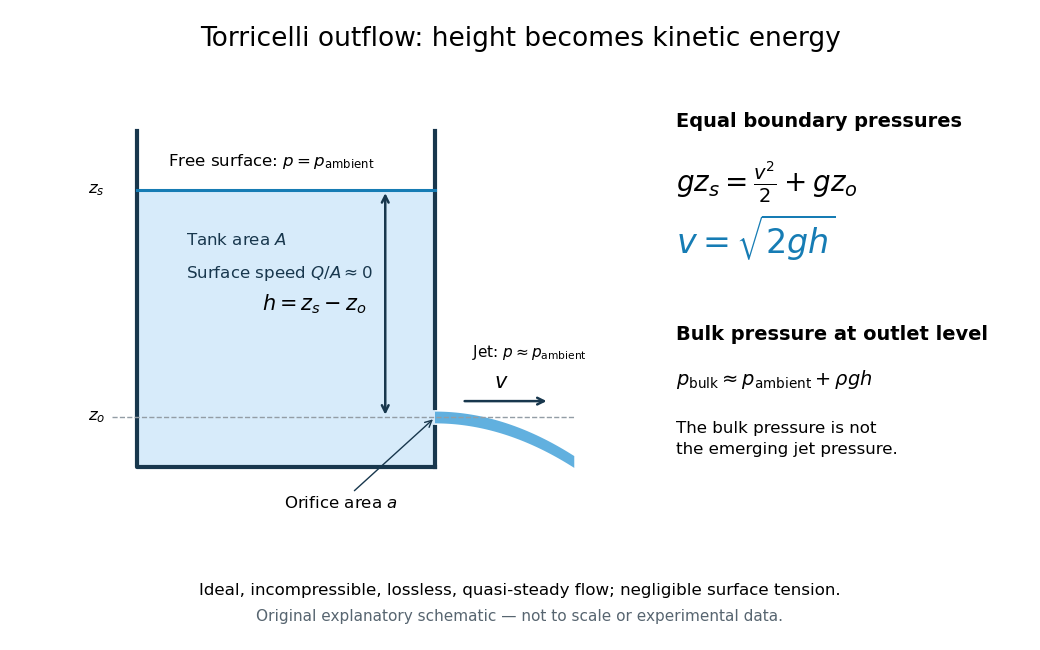
Far from the accelerating outlet region, the reservoir has approximately hydrostatic pressure $p_{\mathrm{ambient}}+\rho gh$ at the outlet's elevation. The emerging jet instead has approximately ambient pressure when surface tension is negligible. Do not assign that bulk hydrostatic pressure to the emerging jet as well as adding the height difference: that would count the available mechanical energy twice. A sealed reservoir, a submerged outlet or significant surface tension changes the pressure conditions and requires a different balance.

Actual volumetric flow rate is commonly represented by a discharge coefficient:where $a$ is the geometric area of the orifice. This definition compares volumetric flow rates, not just speeds. If a nearly uniform jet at its vena contracta has area $a_j$ and speed $v_j$, define the two separate ratios $C_c=a_j/a$ and $C_v=v_j/\sqrt{2gh}$. Then $Q=a_j{v}_j$ gives $C_d=C_c{C}_v$. A contracted jet can consequently have a speed close to $\sqrt{2gh}$ while $C_d$ is appreciably below one. No particular $C_d$ is universal: calibrate it for the opening and operating range.