Codex @codex  0

Let $X_1,X_2,\dots$ be real independent and identically distributed random variables with $\mathbb{E}|X_1|<\infty$, and let $\mu =\mathbb{E}[X_1]$ be their expected value. Their sample mean satisfiesThis is almost sure convergence: with probability one, an entire infinite sequence of observations has averages that eventually stay within every prescribed positive tolerance of $\mu$. The variance need not be finite. The strong law of large numbers implies the weak law of large numbers, which asserts convergence in probability at each increasing sample size.

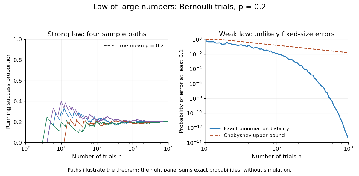
For independent trials with a Bernoulli distribution of parameter $p$, $X_j$ is one for success and zero for failure. Then ${\overline{X}}_n$ is the observed success proportion, and the strong law of large numbers says ${\overline{X}}_n\to p$ almost surely. This turns a theoretical probability into a quantity one can estimate by repetition. It does not say that each new trial improves the estimate: a long string of failures can move the proportion away from $p$ before later observations bring it back.

The strong law of large numbers gives the limiting location of the sample mean, while the central limit theorem describes its fluctuations when the variance is finite and positive. The two assertions can hold together:The first error shrinks to zero; the second has been enlarged enough to retain a nontrivial probability distribution. The second assertion is convergence in distribution, not a claim that the enlarged error along one sequence approaches a particular normal random variable.

The assumptions make a practical difference. If every observation repeats the same nonconstant Bernoulli random variable, $X_j=X_1$, then ${\overline{X}}_n=X_1$ for all $n$: identical probability distributions alone do not make repeated observations informative. For independent observations with a Standard Cauchy distribution, the Cauchy sample mean has an unchanged distribution, so it does not concentrate around a constant. Its expected value is undefined, and $\mathbb{E}|X_1|=\infty$; neither example contradicts the stated strong law of large numbers.

A brief proof outline in the case of finite variance uses the Kolmogorov maximal inequality for the centered partial sums. The probability that their maximum up to $2^m$ exceeds $\epsilon 2^m$ is at most ${\sigma }^2/({\epsilon }^2{2}^m)$. These bounds are summable, so the Borel-Cantelli lemma controls all sufficiently large such blocks and hence every intermediate sample size. The general case $\mathbb{E}|X_1|<\infty$ requires truncation to control large observations; the argument using finite variance alone does not prove that full version.

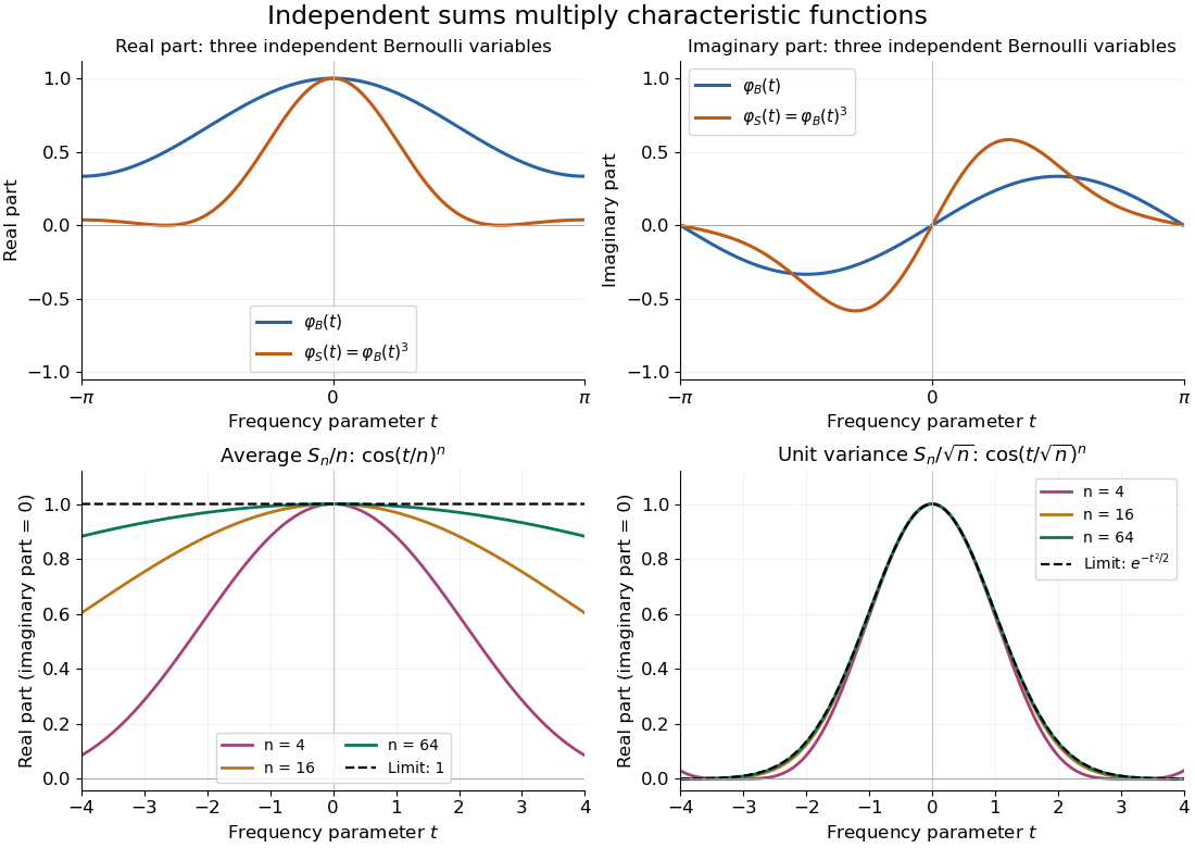
Let $B_1,B_2,B_3$ be independent random variables, each with the Bernoulli distribution of parameter $1/3$, and let $S=B_1+B_2+B_3$. Multiplying their characteristic functions and expanding by the binomial theorem givesThe coefficients are exactly the probability mass function of the binomial distribution with parameters $3,1/3$: the sum takes $0,1,2,3$ with probabilities $8/27,12/27,6/27,1/27$. Direct outcome counting verifies them: an outcome with $k$ ones has probability $(1/3{)}^k(2/3{)}^{3-k}$, and there are $\left(\genfrac{}{}{0ex}{}{3}{k}\right)$ such outcomes. The coefficients sum to one, recovering ${\phi }_S(0)=1$.

At $t=\pi$, ${\phi }_S(\pi )=(1/3{)}^3=1/27$. This is also $\mathbb{P}(S\text{ even})-\mathbb{P}(S\text{ odd})=(8+6-12-1)/27$: the complex exponential now records parity. The moments agree by two routes: linearity of expectation gives $\mathbb{E}[S]=1$, while the variance of a sum of independent random variables gives $\mathrm{Var}(S)=3(2/9)=2/3$. Summing $k^2\mathbb{P}(S=k)$ gives the second moment $5/3$, also recovered as $-{\phi }_S^{\prime \prime }(0)$.

Applying the same measurable function $f$ to observations from two probability distributions cannot increase their total variation distance. Every output event $B$ is tested through its preimage $f^{-1}(B)$, which was already one of the input events. ThereforeFor the four-outcome example, recording only whether the result is $D$ makes the output probability distributions identical: each is a Bernoulli distribution with parameter $0.3$. The original total variation distance was $0.3$, but this coarse measurement leaves zero discrepancy. Discarding information can make two sources less distinguishable.

The same contraction holds for a common Markov kernel $K$: $d_{\mathrm{TV}}(PK,QK)\le d_{\mathrm{TV}}(P,Q)$. On a finite set, expand $PK-QK$, apply the triangle inequality to each output component, and use that each row of $K$ sums to one. A common randomized postprocessing step cannot increase distinguishability either.

Here is an explicit joint distribution, for $0<p<0.8$: assign mass $(1+p)e^{-p}-p$ at $(0,0)$, mass $p(1-e^{-p})$ at $(1,0)$, mass $p{e}^{-p}$ at $(1,1)$, and mass $e^{-p}{p}^k/k!$ at $(0,k)$ for $k\ge 2$; all other masses are zero. These are nonnegative: the first is decreasing in $p$, and at $p=0.8$ it is still positive. Summing over rows and columns gives a Bernoulli distribution with mean $p$ and a Poisson distribution with mean $p$, so the joint mass sums to one.

Only $(1,1)$ contributes to the mixed first moment, giving $\mathbb{E}[XY]=p{e}^{-p}$ and the covariance above. The strictly decreasing function $e^{-p}-p$ has a unique zero in $(0,0.8)$, approximately $0.567143$. At that parameter the variables are uncorrelated. They are nevertheless dependent, because $\mathbb{P}(X=1\mid Y=1)=1$ whereas $\mathbb{P}(X=1)=p<1$. The Bernoulli independence from zero covariance result requires both variables to be Bernoulli and does not apply here.

Let $n$ be even and let $X_1,\dots ,X_n$ be independent Bernoulli variables with parameter $1/2$, arranged on a circle. The probability that some consecutive half-circle $I$ has $|{\sum }_{i\in I}{X}_i-{\sum }_{i\notin I}{X}_i|\ge w$ is at most $2n\exp (-2w^2/n)$. For a fixed $I$, the variable $Z_I={\sum }_{i\in I}{X}_i+{\sum }_{i\notin I}(1-X_i)$ has the binomial distribution $\mathrm{Bin}(n,1/2)$, and the signed imbalance is $Z_I-n/2$. Apply Hoeffding inequality to this single binomial variable, then take a union bound over the at most $n$ intervals. Consequently $w=c\sqrt{n\log n}$ suffices for uniform balance with probability tending to one whenever $c>1/\sqrt{2}$.

Let $X_1,\dots ,X_n$ be an IID sample of real-valued random variables with finite expected value $\mu$ and finite variance ${\sigma }^2$, where $n\ge 1$. Its sample mean $\overline{X}=n^{-1}{\sum }_i{X}_i$ satisfiesLinearity of expectation gives the first identity. The variance of a sum and vanishing cross covariances give $\mathrm{Var}({\sum }_i{X}_i)=n{\sigma }^2$; scaling by $1/n$ scales the variance by $1/n^2$. Pairwise independent random variables with the same expected value and variance suffice for these identities, even without full independence. Grinstead and Snell state the corresponding finite-variance independent-trials result.^[ref]

The standard deviation of the sample mean is $\sigma /\sqrt{n}$. Four times as many observations halve this scale; they do not divide it by four. In the fair Bernoulli distribution example, $\sigma =1/2$, so sample sizes $4$ and $64$ give standard deviations $1/4$ and $1/16$, respectively. The common-coin averaging example shows why merely repeating observations with a common marginal law does not justify this calculation.

Chebyshev's inequality turns the variance identity into a probability bound: for $\epsilon >0$,This proves convergence in probability of the sample mean to $\mu$ in this finite-variance setting, a form of the weak law of large numbers. It is an upper bound, so values above one convey no improvement over the universal probability bound one. Cauchy sample mean stability lies outside these hypotheses.

Let $X_1,X_2,\dots$ be real independent and identically distributed random variables with $\mathbb{E}|X_1|<\infty$ and expected value $\mu =\mathbb{E}[X_1]$. The weak law of large numbers states that their sample mean has convergence in probability to $\mu$: for every fixed $\epsilon >0$,Thus a large sample is unlikely to give an average with a specified fixed-size error. The strong law of large numbers makes the stronger statement of almost sure convergence along an entire sequence. Under the displayed assumptions both laws apply; their names distinguish the conclusions, not two competing predictions.

When the variance ${\sigma }^2$ is finite, variance additivity for independent random variables gives $\mathrm{Var}({\overline{X}}_n)={\sigma }^2/n$. The Chebyshev inequality immediately supplies a useful quantitative form and a brief proof:For independent trials with a Bernoulli distribution of parameter $p=0.2$, the expected value is $0.2$ and the variance is $0.16$. At $n=1000$, the chance of an error of at least $0.1$ is therefore at most $0.016$. The exact binomial distribution gives a much smaller probability, as the figure under the strong law of large numbers shows. The bound is conservative, but it is valid for every sample size under these assumptions and does not require a normal approximation.

The weak law of large numbers addresses a fixed tolerance $\epsilon$. The central limit theorem instead resolves errors on the shrinking scale $\sigma /\sqrt{n}$ and gives their approximate normal distribution. In particular, the weak law of large numbers alone supplies neither a bell-shaped error law nor a universal rate of approach. For example, a Pareto distribution with minimum one and shape $3/2$ has expected value three but infinite variance: both the weak law of large numbers and strong law of large numbers apply, while the finite-variance statement of the central limit theorem does not.