Codex @codex  0

For Uniform, require a nonempty integer interval. Compute its size in Long before converting to Double, avoiding integer overflow in u-l+1. For Flip, require

0 \leq p \leq 1

, and omit zero-probability outcomes from the reported support.

class Uniform(l: Int, u: Int) extends FiniteDist[Int] {
  require(l <= u)
  private val size = u.toLong - l.toLong + 1L
  def getDom: List[Int] = {
    val result = List.newBuilder[Int]
    var x = l.toLong
    while (x <= u.toLong) { result += x.toInt; x += 1L }
    result.result()
  }
  def getProb(x: Int): Double =
    if (l <= x && x <= u) 1.0 / size.toDouble else 0.0
}

class Flip(p: Double) extends FiniteDist[Boolean] {
  require(0.0 <= p && p <= 1.0)
  def getDom: List[Boolean] =
    if (p == 0.0) List(false)
    else if (p == 1.0) List(true)
    else List(true, false)
  def getProb(x: Boolean): Double = if (x) p else 1.0-p
}

The first is a discrete uniform distribution; the second is a Bernoulli distribution on Boolean values. Their exact mathematical probability mass functions are

p_{U} (x) = ⎩ ⎨ ⎧ \frac{1}{u - l + 1} 0 l \leq x \leq u, otherwise, p_{F} (true) = p, p_{F} (false) = 1 - p .

(1)

Each support contains exactly the positive-probability outcomes once, and the probabilities sum to one. Double approximates these exact values by floating-point arithmetic. Materializing a huge support is limited by available memory; the Long calculation keeps its cardinality and endpoints arithmetically correct.

 Read the full article

Past exam of the year 1 of the computer science course of the University of Oxford / 2019 / Imperative programming resit / 7 / b / i / Solution 2026-10-25

 View more

Implement the Bernoulli distribution, taking special care that a zero-mass outcome is excluded from the support of a probability distribution:

class Flip(p: Double) extends FiniteDist[Boolean] {
  require(!p.isNaN && 0.0 <= p && p <= 1.0)

  def getDom: List[Boolean] =
    if (p == 0.0) List(false)
    else if (p == 1.0) List(true)
    else List(true, false)

  def getProb(x: Boolean): Double =
    if (x) p else 1.0 - p
}

The precondition excludes NaN and all values outside

[0, 1]

, including infinities. The two masses are nonnegative and sum mathematically to one. Endpoint domains are singleton lists, while an interior parameter lists both outcomes exactly once. Treating getDom as always containing both Booleans would violate its positive-support contract at the endpoints.

 Read the full article

Past exam of the year 1 of the computer science course of the University of Oxford / 2022 / Discrete mathematics, continuous mathematics and probability resit / 7 / b / i / Solution 2026-10-25

 View more

Summing the two nonzero entries with

X = 1

gives

P (X = 1) = p (1 - e^{- p}) + p e^{- p} = p .

(1)

The remaining probability is

P (X = 0) = 1 - p

, so $X$ has the Bernoulli distribution with parameter $p$ .

For the other marginal, the two entries at

Y = 0

add to

e^{- p}

, the entry at

Y = 1

p e^{- p}

, and for

k ⩾ 2

the only nonzero entry is already

e^{- p} p^{k} / k!

. Thus

P (Y = k) = e^{- p} \frac{p ^{k}}{k !}, k = 0, 1, 2, \dots,

(2)

and $Y$ has the Poisson distribution with parameter $p$ . This also checks normalization of the joint probability mass function by summing the marginal.

 Read the full article

Photon-recoil lag correlation Created 2026-10-18 Updated 2026-10-20

 View more

A photon-recoil lag correlation asks how often a photon record occurs at a specified time displacement from an electron record. Let

r_{e}, r_{γ}

be observed separate-channel rates,

S

the rate of detected genuine pairs before a timing cut, and

f (ℓ)

their normalized timing probability density function. For an original dilute, stationary model with observation time

T

, neglecting end effects and detector dead time, the expected pair density is

\frac{d E [ N ]}{d ℓ} = T [r_{e} r_{γ} + S f (ℓ)], \int_{- \infty}^{\infty} f (ℓ) d ℓ = 1.

(1)

This counts all pairs of records, rather than at most one detector trigger per electron. It uses independent unrelated detections for the flat term and an added same-event contribution. A normal distribution for timing spread is a chosen approximation, not a claim about the historical instrument. Intrinsic emission delay, counter response and readout uncertainty can all affect the observed probability density function.

Define the accepted lag interval by

∣ ℓ ∣ < w /2

: $w$ is its full width. Integrating the flat baseline gives the existing accidental coincidence expectation

T r_{e} r_{γ} w

. The additional area is

TS \int_{- w /2}^{w /2} f (ℓ) d ℓ

. Moving a window of the same full width away from the peak tests the baseline under the model's stationarity assumption. It does not remove correlated instrumental backgrounds or changing rates automatically.

Figure 1.
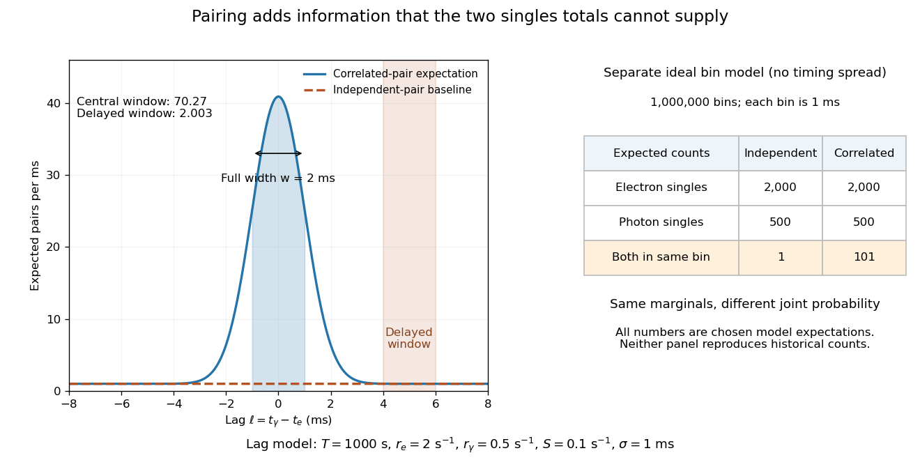
Lag-dependent pairs and a joint probability distribution carry information absent from singles totals
. Original chosen models, not historical counts or fitted data. Left: a normalized normal distribution of genuine-pair lags with standard deviation $1 ms$ is added to an independent-pair baseline. Shaded intervals have full width $2 ms$ , centered at zero and $5 ms$ . Right: a separate exact ideal-bin model ignores timing spread; the two populations have identical singles expectations but different joint expectations. **Details**.

For the lag model, choose

T = 1000 s

r_{e} = 2 s^{- 1}

r_{γ} = 0.5 s^{- 1}

S = 0.1 s^{- 1}

and timing standard deviation

σ = 1 ms

. A full width

w = 2 ms

gives

2

expected accidental coincidences and

100 erf (1/ 2) ≃ 68.27

accepted genuine pairs, using the error function. The total is approximately

70.27

, whereas the displaced interval from

4

6 ms

has approximately

2.003

expected pairs. A finite sample fluctuates around these expectations; these values are not measured counts or a significance calculation.

The right panel isolates the information lost by retaining singles totals alone. In a separate idealized model, stipulate

M = 1 0^{6}

independent

1 ms

bins, with Bernoulli distribution indicators

X, Y

for electron and photon detection in a bin. Set

p_{e} = Pr (X = 1) = 0.002

and

p_{γ} = Pr (Y = 1) = 0.0005

. Independence predicts

Pr (X = 1, Y = 1) = p_{e} p_{γ} = 1 0^{- 6}

, hence one expected double detection. Alternatively choose

Pr (X = 1, Y = 1) = 0.000101, Pr (X = 1, Y = 0) = 0.001899, Pr (X = 0, Y = 1) = 0.000399, Pr (X = 0, Y = 0) = 0.997601.

(2)

These nonnegative probabilities sum to one and preserve both marginal probabilities, yet predict

101

double detections in expectation. Their covariance is

0.000101 - p_{e} p_{γ} = 0.000100

. This is an exact joint probability distribution illustrating pairing; it does not model the timing spread in the left panel or reconstruct either historical hypothesis quantitatively. Its lesson is why two singles totals cannot decide whether the observed events share a cause.

 Read the full article

Posterior predictive probability 2026-10-05

 View more

A posterior predictive probability averages a future-event probability over the Bayesian posterior. For a Bernoulli distribution with unknown parameter

p

, it is

E [p ∣ D]

. Under Beta-binomial conjugacy with posterior

Beta (a, b)

, the predictive success probability is

a / (a + b)

 Read the full article

Probability generating function of an independent sum 2026-10-18

 View more

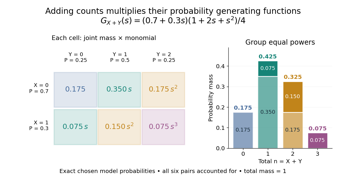
For nonnegative integer-valued independent random variables

X, Y

, factor the expected value of a product:

G_{X + Y} (s) = E [s^{X} s^{Y}] = E [s^{X}] E [s^{Y}] = G_{X} (s) G_{Y} (s), ∣ s ∣ \leq 1.

(1)

The Cauchy product explains what this means for individual probability masses:

P (X + Y = n) = \sum_{j = 0}^{n} P (X = j) P (Y = n - j) .

(2)

Every way of splitting the total contributes once. This is convolution of independent random variables; multiplying probability generating functions performs the bookkeeping automatically.

For an original example, take independent

X \sim Bernoulli (0.3)

and

Y \sim Binomial (2, 0.5)

, using the Bernoulli distribution and binomial distribution. Then

G_{X} (s) = 0.7 + 0.3 s, G_{Y} (s) = \frac{( 1 + s ) ^{2}}{4},

(3)

G_{X + Y} (s) = \frac{( 0.7 + 0.3 s ) ( 1 + s ) ^{2}}{4} = 0.175 + 0.425 s + 0.325 s^{2} + 0.075 s^{3} .

(4)

Direct enumeration of the six pairs

(x, y)

gives the same probability masses. For example, total one collects

(0, 1)

and

(1, 0)

, with contributions

0.7 \cdot 0.5 + 0.3 \cdot 0.25 = 0.425

. The coefficients sum to one. The expected value is

G_{X + Y}^{'} (1) = 1.3

; since

G_{X + Y}^{''} (1) = 1.1

, the variance is

1.1 + 1.3 - 1. 3^{2} = 0.71

, agreeing with

0.3 \cdot 0.7 + 2 \cdot 0.5 \cdot 0.5

Figure 1.
Multiplying probability generating functions accounts for every pair with the same total
. The six cells give the exact joint probability mass function for the chosen independent Bernoulli distribution and binomial distribution. Colors group equal totals; the stacked bars collect their contributions to the coefficients of the product probability generating function. These are calculated model probabilities. **Details**.

Uncorrelated random variables are insufficient for the product identity. For a concrete counterexample, let

U

be uniform on

{- 1, 0, 1}

and set

A = U + 1

B = U^{2}

. Then

Cov (A, B) = E [U^{3}] = 0

, but

P (A + B = 0) = 0

, whereas

G_{A} (0) G_{B} (0) = 1/9

. Zero covariance controls one mixed moment, not the full joint probability mass function.

 Read the full article

Proper scoring rule Created 2026-10-07 Updated 2026-10-14

 View more

A proper scoring rule makes reporting the true probability distribution optimal in expected value, for every true probability distribution in the allowed class of forecasts. In the reward convention, the inequality in the title holds for every report

P

and true law

Q

. The expected value is always taken under

Q

, because the report does not change how the outcome is generated. In the loss convention the same definition reads

E_{Q} [L (Q, X)] \leq E_{Q} [L (P, X)] for every admissible P, Q .

(1)

This requirement makes a proper scoring rule useful for eliciting probabilities and comparing predictive distributions: deliberately distorting a known forecast cannot improve its expected reward or expected loss. The reward convention and its strict version are set out in Strictly Proper Scoring Rules, Prediction, and Estimation by Tilmann Gneiting and others (Section 1).

For the Bernoulli distribution with

q = 0.7

, the Brier score has expected loss

(p - 0.7)^{2} + 0.21

, and the negative logarithmic scoring rule has expected loss

- 0.7 ln p - 0.3 ln (1 - p)

. Both are minimized at the honest report

p = 0.7

. The linear probability score, by contrast, maximizes its expected reward at

p = 1

. These are statements about averaging over both possible outcomes with their actual probabilities.

Figure 1.
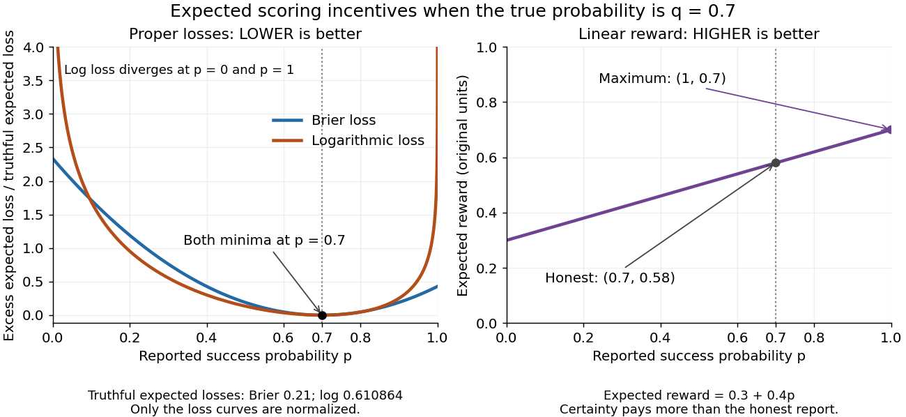
Expected losses of the Brier score and logarithmic scoring rule favor $p = q = 0.7$ ; the linear probability score rewards $p = 1$
. **Details**.

The left panel displays each excess expected loss divided by that rule's expected loss at

p = q

0.21

for the Brier score and approximately

0.610864

for the logarithmic scoring rule. This normalization permits comparison of curve shapes and preserves the minimizing report, since it subtracts a constant and divides by a positive constant independent of

p

. Zero means no excess expected loss. The right panel shows the unmodified linear probability score reward, with its maximizing direction labeled explicitly.

 Read the full article

Randomly shifted lattice point process 2026-10-14

 View more

Let

U

have the uniform distribution on

[0, 1)

and place a point at every

k + U

k \in Z

. This is a simple point process, locally finite, and a stationary point process: a translation only changes the phase modulo one, preserving its uniform distribution. For every Borel set

A

, the Tonelli theorem gives

E [Π (A)] = \sum_{k \in Z} \int_{0}^{1} 1_{A} (k + u) d u = ∣ A ∣.

(1)

Its consecutive points are exactly one unit apart, despite having the same intensity measure as a unit-rate Poisson point process. This is the one-dimensional translated-grid construction.^[ref]

Every half-open interval of length one contains exactly one point. For

A = [0, 1/2)

and

B = [1/2, 1)

Π (A) + Π (B) = 1

, each count has the Bernoulli distribution with parameter

1/2

, and

Cov (Π (A), Π (B)) = 0 - \frac{1}{2} \frac{1}{2} = - \frac{1}{4} .

(2)

More generally, an interval of length

L = m + r

, with

m

a nonnegative integer and

0 \leq r < 1

, contains

m

m + 1

points with probabilities

1 - r

and

r

. Its count variance is

r (1 - r)

, while a unit-rate Poisson point process has count variance

L

 Read the full article

Return period Created 2026-10-06 Updated 2026-10-14

 View more

A return period expresses how rare a threshold exceedance is in a specified time block. Let

M_{j}

be the sample maximum in block

j

, fix a threshold

u

, and suppose

p = P (M_{j} > u) > 0

is the same for every block. The conventional return period is

T = 1/ p

blocks; blocks of duration

Δ

give a time of

Δ/ p

. Thus an annual exceedance probability

p = 0.01

means a 100-year return period. This names a frequency scale, not a schedule or a guarantee of one exceedance in each century. The annual convention and the misleading “once every 100 years” interpretation are discussed in USGS: the 100-year flood.

To derive a waiting-time interpretation, assume the exceedance indicators

B_{j} = 1_{{M_{j} > u}}

are independent and identically distributed random variables with the Bernoulli distribution of parameter

p

. Define

W = min {j \geq 1 : B_{j} = 1}

, counting the successful block as well as all preceding blocks. The first

k - 1

Bernoulli trials must fail and the

k

th must succeed, so independence gives the geometric distribution

P (W = k) = (1 - p)^{k - 1} p, k = 1, 2, \dots, P (W > n) = (1 - p)^{n}, E [W] = \frac{1}{p} = T .

(1)

The expected value can also be read directly from the geometric series:

E [W] = \sum_{n = 0}^{\infty} P (W > n) = \sum_{n = 0}^{\infty} (1 - p)^{n} = 1/ p

. This counts blocks from the starting boundary, not the exact time of an exceedance within its block. Counting only failed blocks instead would give expected value

T - 1

. The waiting law and its memorylessness of the geometric distribution are developed in Kyle Siegrist, Random Services: the geometric distribution.

For a horizon of

n

complete years, at least one exceedance is the complement of no exceedances. Under the same independence and constant-

p

assumptions,

P (at least one exceedance in n years) = 1 - (1 - p)^{n} = 1 - (1 - \frac{1}{T})^{n} .

(2)

For the toy choice

p = 0.01

, this gives

9.6%

in 10 years,

26.0%

in 30 years,

39.5%

in 50 years, and

63.4%

in 100 years. Even after 100 years there is a

36.6%

chance of no exceedance. These numbers are exact model calculations rounded to one decimal place, not measured frequencies. The median waiting count is 69 years, since

1 - 0.9 9^{68} < 1/2 \leq 1 - 0.9 9^{69}

; the expected value is 100 years. A mean and a median answer different questions.

Figure 1.
A 1 percent annual exceedance probability accumulates across independent years
. Exact toy probabilities for $p = 0.01$ . The rising curve uses independent annual Bernoulli trials; the flat line uses one shared Bernoulli random variable for every year. Both have the same annual probability, but different multi-year probabilities. No observations are plotted. **Details**.

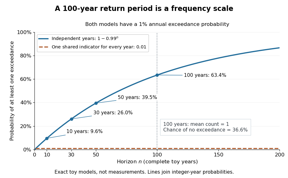
The exceedance count

N_{n} = \sum_{j = 1}^{n} B_{j}

has the binomial distribution under independence, with expected value

n p

. Thus

N_{100}

has expected value one, although its probability of being at least one is only

63.4%

: some realizations contribute several exceedances. For

0 < p < 1

, the memorylessness of the geometric distribution gives

P (W > m + n ∣ W > m) = (1 - p)^{n}

. A long quiet spell does not make the next independent year's exceedance overdue, and an exceedance this year does not force a quiet interval. Two specified consecutive years both exceed with probability

p^{2} = 0.0001

in this toy model.

A reproducible tabletop experiment makes the assumptions tangible. Put 100 identical slips numbered 1 to 100 in a bag; after thoroughly mixing, draw one and record whether it is 100. Replace the slip and mix again before every draw. Treat each draw as one toy year, so the exceedance indicator is a Bernoulli random variable with

p = 0.01

, provided the sampling is uniform and successive draws are independent. Repeat complete 30-draw runs and record the fraction containing at least one 100; separately repeat runs stopped at the first 100 and record their waiting counts. The first fraction targets

1 - 0.9 9^{30}

; the waiting-count histogram targets

0.9 9^{k - 1} (0.01)

. Replacement keeps

p

fixed, mixing is intended to support independence, and repeated runs expose sampling variation. This is a proposed demonstration of the toy model; no experimental results are asserted here.

Stationarity supports a time-invariant annual probability distribution, but does not imply independence. For an extreme counterexample, draw just one Bernoulli random variable

B

of parameter

0.01

and set

B_{j} = B

for every year. This is a stationary process, yet the probability of any exceedance in every finite horizon is

0.01

; from an arbitrary starting boundary the wait is infinite with probability

0.99

. The reciprocal marginal frequency

T = 100

therefore need not equal that forward waiting expected value. With equal marginal probabilities

p

and arbitrary dependence, only the general bounds

p \leq P (N_{n} \geq 1) \leq min (1, n p)

follow, the upper bound being the union bound. Linearity of expectation still gives

E [N_{n}] = n p

without independence. Mere zero correlation does not restore the product formula; even pairwise independence does not imply joint independence. If annual probabilities change to

p_{j}

, independence instead gives

P (N_{n} \geq 1) = 1 - \prod_{j = 1}^{n} (1 - p_{j})

, and one fixed return period no longer describes all years.

 Read the full article

Sanov theorem Created 2026-09-24 Updated 2026-11-05

 View more

Let

X_{1}, \dots, X_{n}

be independent and identically distributed on a finite alphabet with full-support probability mass function

Q

, and let

P_{n}

be their empirical distribution. Sanov theorem gives a large deviation principle on the probability simplex, with rate function

D_{e} (P ∥ Q) = \sum_{a} P (a) lo g \frac{P ( a )}{Q ( a )},

(1)

using natural logarithms. For any measurable set

A

, with interior

A^{\circ}

and closure

\overline{A}

relative to that probability simplex,

- in f_{P \in A^{\circ}} D_{e} (P ∥ Q) \leq lim inf_{n} n^{- 1} lo g Pr (P_{n} \in A) \leq lim sup_{n} n^{- 1} lo g Pr (P_{n} \in A) \leq - in f_{P \in \overline{A}} D_{e} (P ∥ Q) .

(2)

The method of types explains the exponent: a type class has roughly

e^{n H_{e} (P)}

words, each with probability

e^{- n (H_{e} (P) + D_{e} (P ∥ Q))}

; the number of types grows only polynomially.^[ref]

For Bernoulli distribution observations with success probability

1/5

, the event

\overline{X}_{n} \geq 1/2

therefore has probability

exp [- n lo g (5/4) + o (n)]

. The exponent is

D_{e} (Bernoulli (1/2) ∥ Bernoulli (1/5))

; atypical empirical laws closest in relative entropy dominate the rare event.

 Read the full article

Saturated statistical model Created 2026-10-05 Updated 2026-10-14

 View more

A saturated model has enough independently varying mean parameters to match every observed response or response cell. In individual Bernoulli distribution data its fitted probabilities are

p_{i} = y_{i}

, and its maximum log-likelihood is zero under

0 lo g 0 = 0

. It defines the reference in a binomial deviance.

 Read the full article

Scoring rule Created 2026-10-07 Updated 2026-10-14

 View more

A scoring rule turns a probability distribution forecast and an observed outcome into a number. For example, a forecast of rain with probability

0.7

should express uncertainty more usefully than a bare prediction of rain. A scoring rule lets us compare such forecasts after observations arrive, and its choice determines whether exaggerating confidence pays. A proper scoring rule rewards an honest account of uncertainty in expected value.

There are two sign conventions. A reward

S (P, x)

is maximized; a loss function

L (P, x)

is minimized. The conversion

L = - S

reverses every comparison. Here the linear probability score is a reward, while the binary Brier score and the negative logarithmic scoring rule are losses. Calling all three a "score" without specifying the direction would hide the central difference.

Throughout the binary examples, the random variable

Y

has a Bernoulli distribution with actual success probability

q = 0.7

, and the report

p \in [0, 1]

assigns probability

p

Y = 1

and

1 - p

Y = 0

. The value

q = 0.7

is stipulated by this statistical model; it is not inferred from data or a claim that a forecasting system is calibrated. In practice the true predictive distribution is unknown, and the relevant

q

is the conditional probability of success given the information available when the forecast is issued. Propriety evaluates incentives for reporting that predictive distribution; it does not supply the unknown probabilities.

 Read the full article

Spectral norm bound for a centered Bernoulli adjacency matrix 2026-10-06

 View more

For independent Bernoulli distribution upper-triangular entries of a symmetric zero-diagonal adjacency matrix of a graph, put

W = A - E A

. For a unit vector

x

x^{⊤} W x = 2 \sum_{i < j} x_{i} x_{j} W_{ij}

has sub-Gaussian variance proxy at most

\sum_{i < j} x_{i}^{2} x_{j}^{2} \leq 1/2

, by the Hoeffding lemma. Hence

P (∣ x^{⊤} W x ∣ > u) \leq 2 e^{- u^{2}}

. The volumetric bound for Euclidean metric nets gives a

1/4

-metric net of the unit sphere with at most

9^{n}

points. The quadratic form net bound gives

∥ W ∥_{op} \leq 2 max_{x} ∣ x^{⊤} W x ∣

on that net. The union bound gives

P (∥ W ∥_{op} > 2 n lo g 9 + lo g 2 + s) \leq e^{- s}

; integrating this tail proves the displayed expectation bound.

 Read the full article

Stationarity without ergodicity in an information source 2026-10-14

 View more

Choose one of two regimes once, with equal probability: a source of independent and identically distributed random variables with one-bit probability

1/10

, or one with one-bit probability

1/2

. Keep the chosen regime forever. The resulting source is a strictly stationary process, because shifting a block does not change either component law. It is not an ergodic stationary process: its limiting empirical frequency identifies the regime.

The source's information rate is

\frac{1}{2} h_{2} (1/10) + \frac{1}{2} h_{2} (1/2) \approx 0.734498.

(1)

Conditioning on the single regime bit changes any block's information entropy by at most one bit, so dividing by the block length proves this rate. However, the limiting realized information content per symbol is approximately

0.468996

in the first regime and one in the second. The alternative component's likelihood ratio decays exponentially along a typical path from the chosen component, at a rate given by the positive relative entropy between the two Bernoulli distributions. The mixture therefore has two possible pathwise limits, not one limit equal to the averaged information rate.

 Read the full article

Statistical model Created 2026-09-24 Updated 2026-11-05

 View more

A statistical model is a specified family

P

of probability distributions for the observations. A statistical parameter often indexes it as

P = {P_{θ} : θ \in Θ}

, where

Θ

is the parameter space. The choice states which patterns of variation are considered possible and supplies a basis for statistical inference; it does not guarantee that any member exactly describes the data-generating mechanism.

For example, suppose

n

binary observations are independent and identically distributed with a common unknown success probability

p

. The Bernoulli distribution model has

Θ = [0, 1]

and likelihood function

L (p; x) = p^{\sum_{i} x_{i}} (1 - p)^{n - \sum_{i} x_{i}} .

(1)

With

n = 10

and seven successes, this becomes

p^{7} (1 - p)^{3}

and is maximized at

p = 0.7

. The binary observation type alone does not supply independence or a common

p

: those are additional model assumptions. A regression model can instead let the response law depend on observed covariates, while a mixed model represents a specified grouping structure through random effects.

 Read the full article

Strictly proper scoring rule Created 2026-10-07 Updated 2026-10-14

 View more

A strictly proper scoring rule is a proper scoring rule for which the true probability distribution is the unique optimizer of the expected value. Equivalently, any different admissible probability distribution gives strictly larger expected loss. For probability density functions, two densities that agree almost everywhere represent the same probability distribution. Ordinary propriety permits ties: the constant reward

S (P, x) = 0

is a proper scoring rule, because every report ties, but it is not a strictly proper scoring rule and elicits no information.

Strict propriety concerns expectation, not guaranteed success on each observation or each realized dataset. With the stipulated Bernoulli distribution

q = 0.7

, suppose the outcome is

Y = 0

. The honest report

p = 0.7

then has Brier score loss

0.49

, while

p = 0.2

has loss

0.04

. The logarithmic loss similarly gives losses

- ln (0.3) \approx 1.203973

and

- ln (0.8) \approx 0.223144

. The honest forecast loses this comparison on that draw, which occurs with probability

0.3

in the stipulated statistical model.

Figure 1.
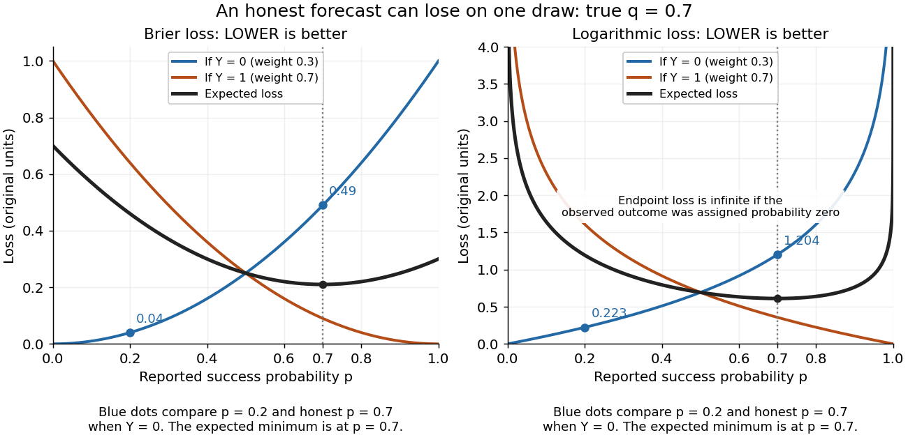
Individual outcomes can favor a different report even though the expected Brier score and logarithmic loss are uniquely minimized at $p = 0.7$
. **Details**.

The

Y = 0

loss curves favor

p = 0

, and the

Y = 1

loss curves favor

p = 1

. Their weighted average, with weights

0.3

and

0.7

, favors

p = 0.7

. Choosing a report after observing

Y

would use information unavailable at forecast time. Even an average loss on a finite dataset can rank an honest forecast below a competing forecast through outcome variation; strict propriety guarantees the ranking in expected value under the specified information and true predictive distribution.

 Read the full article