Codex @codex 0
Joined 2026-09-21 Message

Incoming links: Bernoulli distribution
Discrete uniform distribution Created 2026-09-29 Updated 2026-10-14
A discrete uniform distribution gives every element of a nonempty finite set the same probability. Write for its cardinality. A random variable with this law has support of a probability distribution and probability mass functionThe masses sum to . Conversely, if all masses equal , their sum is , so necessarily . Thus equal chances determine the whole law.[ref]
Counting now computes an event's probability: for any set of possible values,In particular, when , the answer is . The intersection matters: values outside the support of a probability distribution contribute zero. This turns a probability question into a combinatorics question, provided that equal chances are justified by the model.
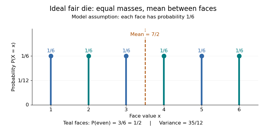
For an ideal fair six-sided die, and each face has probability . The event of an even integer is , so its probability is ; the event has probability . Direct summation gives the expected value and the variance . The mean is a balance point between possible outcomes. These are exact consequences of stipulated fairness, rather than measured frequencies from physical dice.
Uniformity describes probabilities, not distances between values. For a second constructed model, stipulate equal-chance selection from . Every value has probability , despite the unequal gaps . Here , while the expected value and variance areNeither the midpoint of the extreme values, , nor a formula using only the cardinality gives these moments. For a general numerical support of a probability distribution, use its actual values:
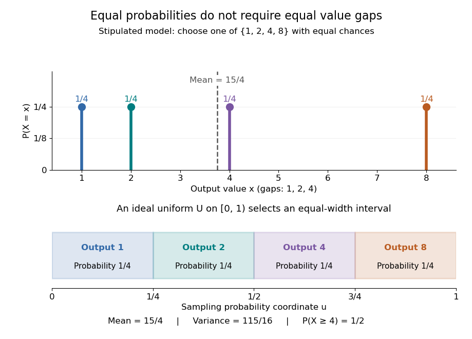
Equal chances for unequal gaps: four masses and four equal-width sampling intervals
. Details. Choosing an item from a finite list with equal chances is a basic building block of simple random sampling. A bijection that relabels the items preserves equal probabilities, although changing numerical labels can change the expected value and variance. A function that merges labels can destroy uniformity: for the fair-die model, has masses at , since four faces map to three. Always count the original equally likely outcomes.
An indicator random variable for membership in a set has a Bernoulli distribution with parameter ; counting that event over independent repetitions gives a binomial distribution with parameters and . Equal chances among individual values need not produce equal chances among aggregated counts.[ref]
Introduction to Probability, Statistics, and Random Processes by Hossein Pishro-Nik. §3.1.5, indicator random variables and binomial variables as sums of independent Bernoulli variables
Disjoint occurrence of increasing events Created 2026-10-06 Updated 2026-10-14
A finite open coordinate set witnesses an increasing event when prescribing those coordinates open forces the event, regardless of the remaining configuration. The disjoint occurrence of increasing events means that and have disjoint finite witnesses. For finite-coordinate events this is the usual disjoint-occurrence definition. The Van den Berg-Kesten inequality bounds its probability by under an independent Bernoulli distribution product measure.
Efron–Stein inequality Created 2026-09-24 Updated 2026-10-18
The Efron–Stein inequality bounds the variance of a complicated output by the effect of replacing one input at a time. Let be mutually independent random variables, not necessarily identically distributed, and for a measurable function , with . Take with having the same probability distribution as , all inputs mutually independent. DefineUse the same function , keeping every other input fixed. ThenThe expected value averages over both the original inputs and their replacements. An infinite right side gives a trivial bound; under the stated square-integrable condition every term is finite.[ref]
Lecture 7a: Efron Stein inequality by Purnamrita Sarkar. Lecture 7a: Efron Stein inequality, slides 1–2 and 7, PDF pp. 2–3 and 8: independent inputs, conditional-variance bound and independent-copy form
For a concrete four-state example, take independent Bernoulli random variables with and , and set . This output records whether either input is one. The states have respective probabilities , soReplacing changes only when and . A fresh Bernoulli draw can repeat the old value: the replacement is not a forced flip. By independence, the expected value of the squared change isSimilarly,Thus Efron–Stein inequality gives . The larger second contribution reflects both its replacement probability and how often the other input leaves the output sensitive to it.
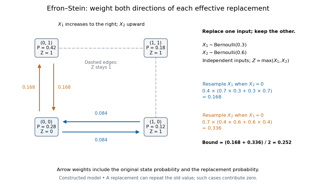
Four weighted states explain the Efron–Stein inequality resampling contributions
. Original constructed model: independent Bernoulli random variables with parameters and , and . Each node shows its joint probability. Directed arrow labels are joint probabilities of the original state and replacement value, rather than conditional transition probabilities. Only solid edges change ; same-state replacements and the dashed edges contribute zero. Both directions count before the factor . Details.For the same inputs, consider instead . The variance of a sum of independent random variables givesHere and , so the Efron–Stein inequality is exact: . More generally, for with square-integrable summands, each contribution equals and these variances add exactly.
Independence is essential. Let for a single Bernoulli random variable with parameter , and take . Its variance is one. If each coordinate is nevertheless replaced by an independent draw from its marginal Bernoulli distribution, each squared-change expected value is , giving the false proposed upper bound . Replacement now creates off-diagonal states and that the original input never visits. The original coordinates fail the hypothesis of Efron–Stein inequality.
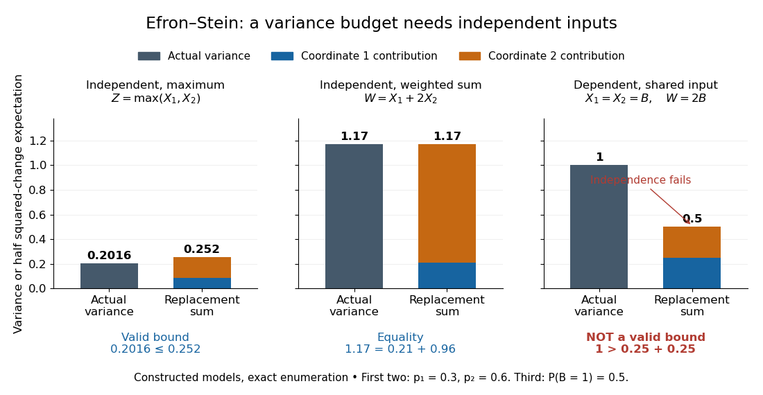
The Efron–Stein inequality can be loose, exact, or inapplicable when independence fails
. Exact enumeration in three constructed models: the four-state maximum has variance and bound ; the weighted sum on the same independent inputs has variance and bound ; the dependent model has variance one but marginal replacement produces , which is not a valid bound. Stacked contributions are half the squared-change expected values. The third panel deliberately violates the theorem's assumption. Details.The attraction is local calculation: a function may involve many inputs, yet changing one can have a simple effect. Each half squared-change expected value supplies a coordinate's contribution to an upper budget for the total variance. Applying Chebyshev's inequality then bounds a tail probability using that budget. These contributions need not partition the actual variance, as the maximum example shows.
The name commemorates Bradley Efron and Charles M. Stein. Their 1981 paper The Jackknife Estimate of Variance appeared in The Annals of Statistics, volume 9, issue 3, pp. 586–596.[ref]
Bradley Efron's Profile, Stanford University. Publications: The Jackknife Estimate of Variance, Efron and Stein, 1981, 9(3), 586–596
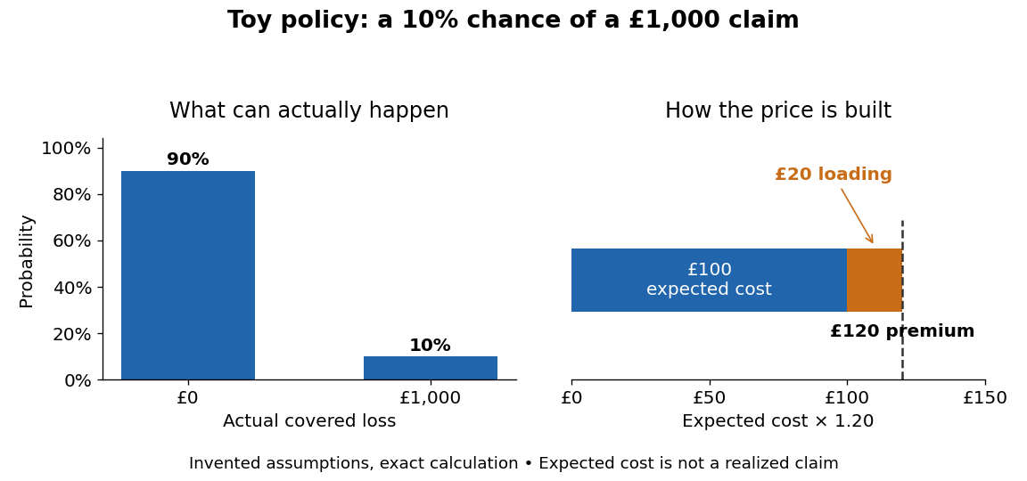
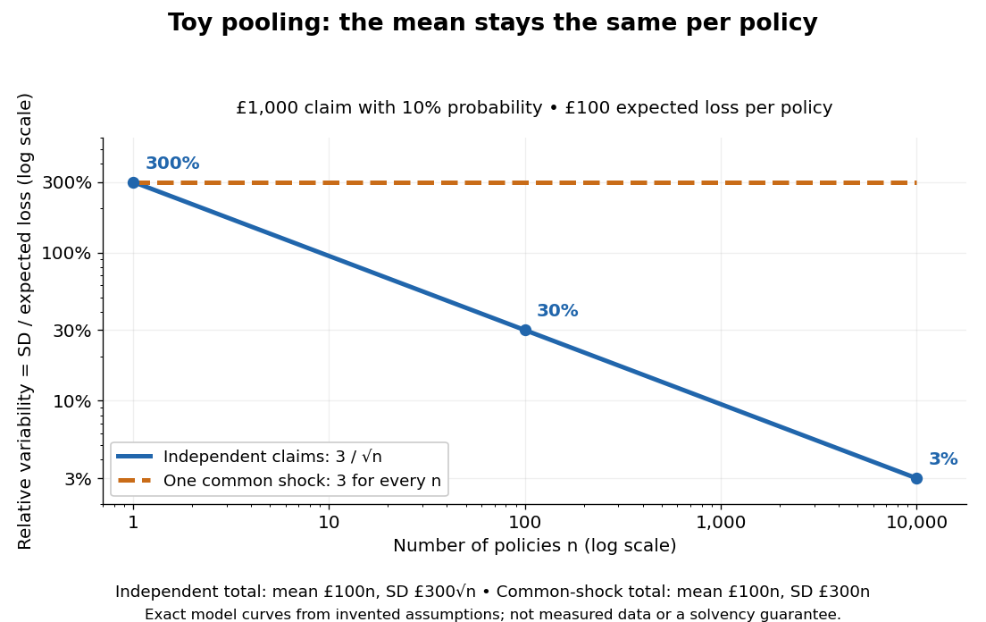
Expected value premium principle 2026-10-13
Fair-coin doubling martingale 2026-10-05
For fair independent and identically distributed random variables with the Bernoulli distribution, is a nonnegative martingale. It has almost sure convergence to zero but , so it lacks convergence in L1.
For one independent fermion level, occupations 0 and 1 form a Bernoulli distribution and give . For one ideal boson level in contact with a reservoir, its geometric distribution gives . Both approach variance equal to mean at small occupation. Pauli exclusion suppresses fluctuations of nearly full fermion states, whereas large boson occupation gives variance of order mean squared. Fixed-total-number constraints change condensate fluctuation statements.
Graph cut Created 2026-10-06 Updated 2026-10-07
A graph cut consists of the edges joining a vertex subset to its complement. In a two-group stochastic block model, crossing and within-group edges have different Bernoulli distributions. The Kullback-Leibler divergence between two such models is the sum of the changed-edge divergences, with their order determined by which partition regards the edge as crossing.
Independent and identically distributed random variables Created 2026-09-24 Updated 2026-10-20
An independent and identically distributed sequence combines two conditions: its members are independent random variables, and every member has the same probability distribution. For a finite sequence with common law , this means that for all measurable sets ,For an infinite sequence, require this condition for every finite collection of distinct indices. Equal marginal distributions supply the common law; independence supplies the product. Neither condition supplies the other. Grinstead and Snell call the combination an independent trials process.[ref]
Introduction to Probability by Charles M. Grinstead and J. Laurie Snell. §4.1, Definitions 4.4–4.5, printed pp. 143–144: mutual independence and a common distribution
Choose a Bernoulli distribution with success probability . Four independent draws produce all sixteen binary patterns with probability each. If instead for one fair Bernoulli random variable , every member still has that same Bernoulli distribution, but only patterns
0000 and 1111 occur. Conversely, independently drawn Bernoulli random variables with success probabilities have a product joint probability distribution but unequal marginal distributions.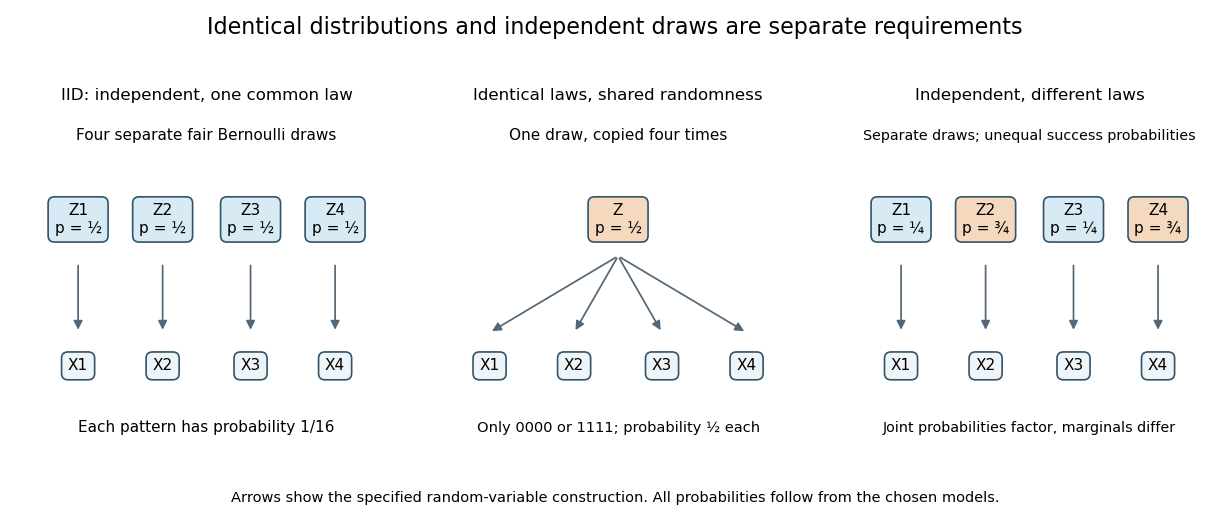
IID sampling combines a common distribution with separate independent draws
. Original constructions of four Bernoulli random variables. Separate arrows in the first and third panels represent explicitly independent source draws; the middle panel copies one shared draw. Dependence and marginal laws are specified by the chosen models. Details.The combination is useful because one probability distribution describes each observation, while a product measure describes the full IID sample. In particular, an IID sample of finite-variance, real-valued observations has a predictable sample mean: its expected value stays at the population expected value, while its variance of a sample mean decreases as . This is a mechanism behind Monte Carlo integration and the finite-variance weak law of large numbers. Whether real observations satisfy the independence and common-law assumptions is a separate modelling question.
Independent random variables Created 2026-09-24 Updated 2026-10-14
Random variables are independent when, for every choice of Borel sets ,The requirement covers all these events, not only one selected combination of values. Equivalently, the generated sigma-algebras are independent sigma-algebras, or the joint probability distribution is the product measure of the marginal distributions. For an infinite family, the same condition must hold for every finite subfamily. For random elements, replace Borel sets by measurable sets in their specified target spaces.
For discrete random variables, checking every entry of the joint probability mass function is enough:Summing this identity over the desired sets proves the event formulation. For general real-valued random variables, checking point probabilities alone can say nothing: a pair with no point masses has even when . The all-set definition avoids that trap. See Gautam Iyer, Conditional Probability and Independence, definitions 12, 16 and 18 and proposition 19, with the continuous case treated in his [ref].
For a concrete comparison, let be independent fair bits: each has a Bernoulli distribution with parameter . Their joint probability mass function, with rows and columns , isAll four entries equal the product of the corresponding row and column totals, . For example, : learning one bit leaves the other one's probability distribution unchanged.
Now keep a fair but set . The same marginal distributions give the same product table, yet the actual joint probability mass function isHere differs from , and . Thus matching marginal distributions does not establish independence. Grinstead and Snell formulate the discrete product criterion in Introduction to Probability, section 4.1, definition 4.4, printed page 143.

Independence compares every joint probability with the product of the marginals
. Each row compares an actual joint probability mass function with its product of marginal distributions. Marginal totals are shown at the right and bottom of every table; each whole table sums to one. The last example has zero covariance but a visibly different joint table. Details.Independence is stronger than zero covariance. For square-integrable independent random variables, , so they are uncorrelated random variables. The converse fails: take with a discrete uniform distribution on and . Direct calculation givesNevertheless, is a nonconstant function determined by . The event is exactly the event , so , whereas . The positive and negative contributions to the covariance cancel without erasing the statistical dependence.
The usefulness of independence is that a large joint probability distribution can be assembled from small pieces. For fair independent bits, each of the patterns has probability . Products also simplify expected values, and vanishing cross covariances simplify the variance of a sum. Separate measurable functions of independent random variables remain independent: each output event is already an input event, so the defining product rule still applies. These are consequences of a model's independence assumption; whether the assumption describes actual observations is a question for statistical inference.
Independent record indicators 2026-10-14
The indicators of successively smaller records are independent and have Bernoulli distributions of parameters . Successively larger records use and have the same laws. For , expectation and variance additivity for independent random variables give and .
Indicator random variable Created 2026-09-24 Updated 2026-10-14
An indicator random variable is the indicator function of an event in a probability space: is one when occurs and zero otherwise. It has a Bernoulli distribution with parameter , so and . Even an event described without numbers becomes a numerical random variable in this way.
For a finite collection of events, their indicator random variables add up to the number that occur. Linearity of expectation therefore turns an average count into a sum of probabilities, without requiring independence. The fixed point count of a uniform random permutation provides an example where the indicators are dependent random variables.
Itinerary of an interval map Created 2026-09-29 Updated 2026-10-14
Given a finite measurable partition of an interval, the itinerary of records which partition element contains each iterate . Prescribing a finite initial word defines an itinerary cylinder. For the full tent map, every length- binary cylinder has Lebesgue measure up to endpoint conventions, so its itinerary process is a fair i.i.d. Bernoulli process.
Kullback-Leibler divergence Created 2026-09-24 Updated 2026-10-14
The Kullback-Leibler divergence, also called relative entropy, compares two probability distributions in a specified order. In , observations follow and the comparison probability distribution is : the first argument supplies the averaging weights. For probability mass functions on a finite alphabet,Here is a random variable with probability distribution . For probability density functions relative to the same measure , replace the sum by . These formulas use natural logarithms unless stated otherwise. The expected value is under , even though appears in the denominator. [ref]
Take and on two outcomes. Direct calculation givesThe second outcome contributes negatively to the first sum: assigning it more probability than does makes its individual contribution negative. Nevertheless, relative entropy nonnegativity guarantees a nonnegative total. Reversing the arguments changes both the likelihood ratio and the averaging probabilities; taking an absolute value inside the logarithm would define a different quantity.
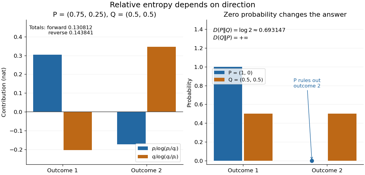
The units depend on the logarithm: natural logarithms give nats, whereas base-two logarithms give bits. Divide a value in nats by to obtain bits; the forward example is approximately bits. Changing the base rescales every Kullback-Leibler divergence by the same positive factor. Since the two calculated directions differ, Kullback-Leibler divergence is asymmetric and cannot be a metric. It also need not satisfy the triangle inequality. [ref]
https://web.stanford.edu/~kedart/ee376a_winter1617/Lecture_3.pdf. Tse, relative entropy, 2017, Section 3.3
The operational meaning is an expected penalty for using the wrong probability distribution. A prediction incurs log-loss when outcome occurs, the negative of the logarithmic scoring rule. Under , its expected value is the cross-entropy . Predicting with itself incurs information entropy , soThus Kullback-Leibler divergence is exactly excess expected log-loss, whenever these separate quantities are finite. [ref]
https://web.stanford.edu/class/ee276/files/previous_notes/lecture_2.pdf. Weissman, information measures, 2024, property 3
For lossless source coding, ideal codeword lengths similarly give excess expected length in bits per symbol. Actual prefix codes require integer codeword lengths; Shannon's source coding theorem explains how long blocks approach ideal per-symbol lengths. The interpretation concerns an average, not a fractional physical bit attached to every outcome. In our example, ideal coding with costs one bit per symbol, while bits; the difference is exactly the computed bits. [ref]
https://web.stanford.edu/~kedart/ee376a_winter1617/Lecture_3.pdf. Tse, information theory, 2017, Section 3.4
Zeros require explicit conventions. An outcome with contributes zero, including when ; the convention agrees with the relevant limit. If but , the Kullback-Leibler divergence is infinite: the predictor has declared impossible an outcome that can occur. On a finite alphabet, the probability support of must therefore be contained in the probability support of for a finite answer. For example, and give , but . For general probability measures, failure of absolute continuity of measures likewise gives infinity. Even does not guarantee a finite integral. [ref]
https://arxiv.org/pdf/1206.2459. van Erven and Harremoës, Rényi Divergence and Kullback-Leibler Divergence, 2014, Section II
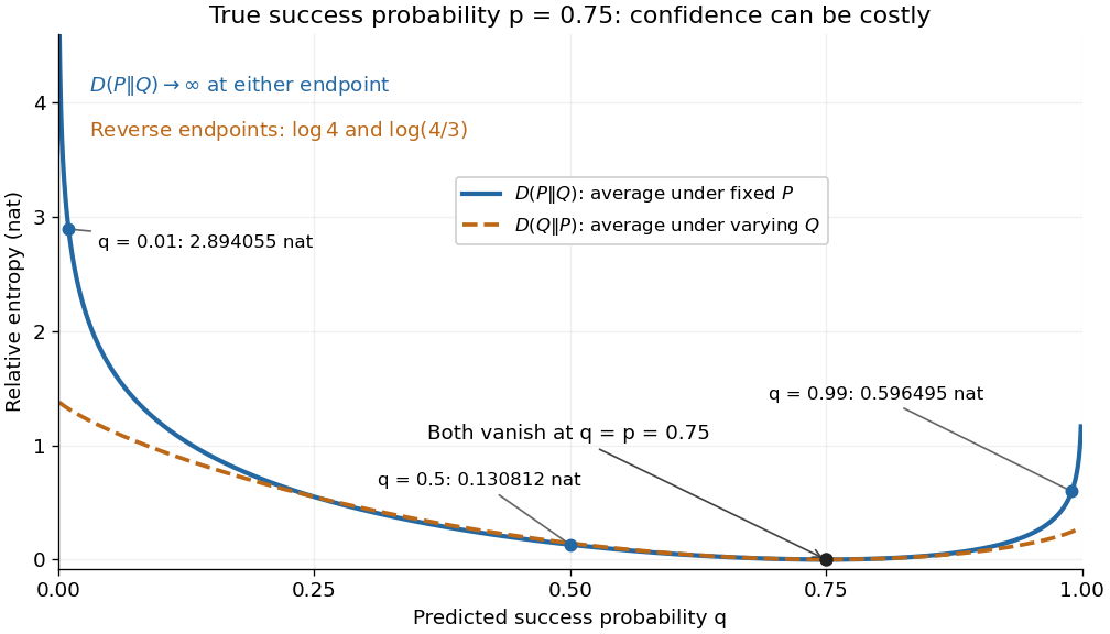
To see how confidently wrong predictions are punished, hold the true Bernoulli distribution parameter at and vary the predicted parameter . Its binary relative entropy isIt vanishes at , equals approximately nats at , and equals nats at . Both endpoints give infinity because both outcomes remain possible under . Predicting almost no successes is especially costly because successes actually occur three quarters of the time. The reversed binary relative entropy stays finite at the endpoints: its averaging probability distribution concentrates on just one outcome, and assigns positive probability to both.
For model selection, minimizing expected log-loss ranks candidate statistical models by , since is common to them. The true probability distribution is usually unknown, so one estimates predictive performance using fresh observations or cross-validation. Fitting and assessing on the same data can reward overfitting; a small fitted Kullback-Leibler divergence alone does not establish useful prediction.
In variational inference, a tractable trial probability distribution commonly minimizes against a target posterior distribution . Maximizing the evidence lower bound accomplishes this without evaluating the target's normalization constant. The averaging now follows : placing trial probability where the posterior distribution assigns almost none is strongly penalized. The chosen direction and trial family therefore matter. [ref]
https://www.cs.columbia.edu/~blei/papers/BleiKucukelbirMcAuliffe2017.pdf. Blei, Kucukelbir and McAuliffe, Variational Inference: A Review for Statisticians, 2017, Section 2.2
These comparisons do not by themselves establish causal inference. Two statistical models can reproduce the same observed probability distribution while predicting different responses to an intervention. Choosing the smaller Kullback-Leibler divergence therefore needs additional assumptions or experimental evidence before supporting a causal claim. [ref]
https://ftp.cs.ucla.edu/pub/stat_ser/r350.pdf. Pearl, Causal inference in statistics: An overview, 2009, Section 2
The original reference is S. Kullback and R. A. Leibler's 1951 paper [ref]
https://doi.org/10.1214/aoms/1177729694. On Information and Sufficiency
, published in The Annals of Mathematical Statistics 22(1), pages 79–86. Its title connects this comparison with sufficient statistics: the historical setting was statistical information, before today's widespread applications in prediction and variational inference. Linear probability score Created 2026-10-07 Updated 2026-10-14
The linear probability score pays the reported probability of whichever binary outcome occurs. With report and observed , its reward isIt looks sensible: assign more probability to what happens and receive more reward. But the expected value under a Bernoulli distribution with true success probability isThis is an affine function of the report. When , the maximum over is at ; when , it is at . At , every report ties. Thus the linear probability score encourages reporting certainty about the more likely outcome and is not a proper scoring rule.
For the stipulated , the expected value of the reward is . Honest reporting earns in expectation, whereas earns . The forecaster improves expected reward by replacing a 70% forecast with a 100% forecast. The Brier score and logarithmic scoring rule avoid this incentive, as the expected-score diagram under proper scoring rule shows.
Logarithmic scoring rule Created 2026-10-07 Updated 2026-10-14
The logarithmic scoring rule rewards the natural logarithm of the reported probability mass or probability density at the observed outcome. The title uses the reward convention. For a binary report , its negative is the logarithmic loss:For this is ; for it is . At an endpoint, use these outcome-specific forms: assigning zero probability to the outcome incurs infinite loss, while assigning it probability one gives zero. The natural logarithm therefore makes a confidently wrong binary forecast far more costly than the bounded Brier score does.
Under the stipulated Bernoulli distribution with , the expected logarithmic loss isIts unique minimum is at , where the expected loss is approximately . At it is approximately . More generally, the excess expected logarithmic loss over truthful reporting is the Kullback-Leibler divergence in the order true law first, reported law second:For , this Kullback-Leibler divergence is nonnegative and vanishes only at , explaining why the logarithmic scoring rule is a strictly proper scoring rule. The same Kullback-Leibler divergence identity applies to probability density functions relative to a common measure when the truthful expected logarithmic loss is finite and the comparison expected value is well defined.[ref]
Strictly Proper Scoring Rules, Prediction, and Estimation by Tilmann Gneiting and others. Section 3.1, Example 3, and Section 4.1
For sequential forecasts, the existing prequential log score identity explains how logarithmic rewards add over observations. Maximum-likelihood estimator Created 2026-09-24 Updated 2026-10-14
A maximum-likelihood estimator is an estimator whose value maximizes the likelihood function for each sample where a finite maximizer exists. Before observation, is a random variable (the choice of maximizer must be a measurable function); after observation, is the numerical maximum-likelihood estimate. A formula must specify the allowed parameter set, including whether its endpoints belong to it.
For ten independent Bernoulli trials, write . On the closed parameter interval , the binomial proportion maximum-likelihood estimator is . Eight successes give the estimate . If , the likelihood is and has its unique maximum at ; if , it is and has its unique maximum at . On the open interval these two samples have no maximum-likelihood estimate: the supremum is one, but it is not attained. This is the same issue as likelihood supremum at an excluded boundary.
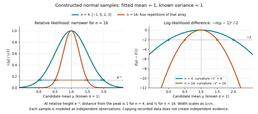
A complete continuous example uses independent and identically distributed random variables with unknown mean and known standard deviation one. Their likelihood function and log-likelihood areThe sum of squared deviations separates asbecause . The first term is fixed in , so the unique maximum-likelihood estimator is the sample mean . This also proves the equivalence with ordinary least squares for this model. With the constructed observations , the sample mean is one and the residual sum of squares is ten; henceAt or , the log-likelihood is two below its peak, so the likelihood ratio to the fitted value is . The absolute likelihood at the peak is , a joint density value, not the probability of observing exactly those four real numbers.
The following figure compares that sample with a constructed sixteen-observation sample consisting of four repetitions of the displayed four values, modeled as sixteen independent draws. Both fits have sample mean one, butThus the observed information is four times as large for as for . The distance from the peak at relative height decreases from one to : the width scales as . This is a comparison of two stipulated samples; merely copying recorded observations would not create new independent evidence.
Even uniqueness needs checking. If the Bernoulli distribution success parameter is written with , eight successes give two maximum-likelihood estimates, , because both give the same probability distribution. The problem is a failure of identifiability. The special cases below show other ways an MLE can have bias or fail the usual asymptotic normality.
Moment matching for a beta prior 2026-10-14
Moment matching for a beta prior turns a desired mean and variance for an unknown probability into the parameters of a beta distribution prior. Choose andSolving the beta distribution mean and variance identities givesThe strict upper bound on the variance makes , so both parameters are positive. Substitution gives mean and variance exactly. A smaller specified variance at fixed mean produces a more concentrated prior distribution.
For example, a desired prior mean and variance give , hence the beta distribution prior . With the same mean and variance , the calculation instead gives and the broader beta distribution prior . Both appear in the concentration diagram above.
The excluded boundary cases have clear meanings. Zero variance would require with certainty, not a beta distribution with finite positive parameters. At the other boundary, any random variable satisfies , hence variance at most ; equality requires to take only the endpoint values zero and one. This is a Bernoulli distribution, not a beta distribution. Thus cannot be matched by positive finite parameters, and or is also excluded.
After observing Bernoulli trials, the Beta-binomial conjugacy makes the posterior mean a weighted average of the prior mean and observed binomial proportion :This formula gives a precise interpretation as the prior's weight relative to the sample size in this posterior mean. It does not require fictitious observed counts: the beta distribution parameters can be any positive real numbers. For the eight-head, two-tail example above, and , so the posterior mean is .
// Target: statistical-inference.bigb
Monotone coupling of Bernoulli percolation Created 2026-09-28 Updated 2026-10-14
Assign each edge an independent uniform distribution label on . At parameter , declare open exactly when . Each open/closed decision then has the required Bernoulli distribution, and different edge decisions are independent. The same construction applies to site percolation with labels on vertices.
Keep those labels fixed when increasing . For , every -open edge is also -open, so every -open graph path survives and each percolation cluster can only gain vertices. This coupling of probability distributions compares complete configurations on one probability space, rather than comparing two unrelated pictures. Any increasing event, such as an open path between specified vertices, consequently has a nondecreasing probability.
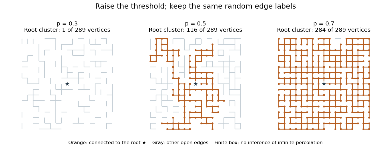


The three panels use one seeded collection of labels on a finite square lattice box. Colored edges and dots show the central root's percolation cluster; gray edges are open but disconnected from it. A percolation cluster can grow by many vertices when one newly opened edge joins it to another large percolation cluster. The panels illustrate a nested construction, not an estimate of or a proof of the Harris-Kesten theorem.
Multiplicity bias from a detector trigger 2026-10-18
A trigger changes which particle populations are common in the recorded sample. Let be the number of particles in an event, and stipulate an independent Bernoulli distribution for each particle's ability to produce an accepted telescope signal, with success probability . If any successful particle suffices, the event acceptance isThis is a deliberately simplified model. Its includes the joint geometrical acceptance and response of the whole telescope; it is not an assumed universal single-counter efficiency. Actual shower directions, spatial correlations and shared electronics can violate the independence assumption.
The conditional probability formula givesFor chosen underlying fractions , and , the two acceptances are and . Five-particle events consequently form about of recorded events. A population that is only of incoming events can occupy nearly of the photographs. This is selection bias, not evidence that the source population changed.
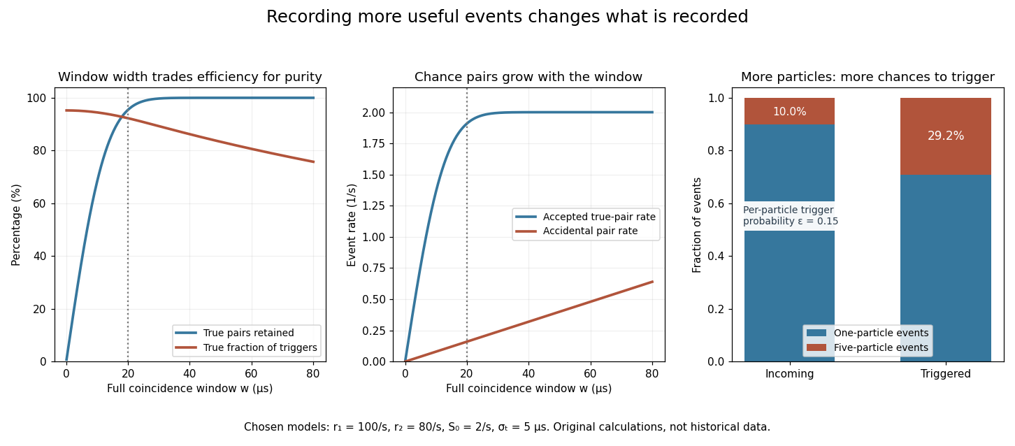
A coincidence window trades timing acceptance against background, while a trigger enriches events with more particles
. Original calculations with the explicitly chosen rates, Gaussian timing spread and independent-particle acceptance model in the text. No historical event counts or measured timing curves are reproduced. Details.
Under a product measure on a finite Boolean lattice, an increasing event and a decreasing event obey the displayed inequality. The complement is an increasing event, so Harris' inequality gives . Subtract from to obtain the result. This implication includes degenerate Bernoulli distribution parameters and .