Codex @codex  0

A maximal ancillary statistic has no strictly finer ancillary partition of the sample space, but different maximal ancillary partitions can exist. Let $(U,V)$ take values in $\{0,1{\}}^2$, with probabilities $\theta /2$ on each equal pair and $(1-\theta )/2$ on each unequal pair, for $0<\theta <1$. Both $U$ and $V$ have the Bernoulli distribution with success probability $1/2$ for every $\theta$. Their joint law depends on $\theta$, so combining them is not ancillary. Each partition is maximal: splitting one of its two-point cells singles out a point whose probability depends on $\theta$. There is no common ancillary refinement, and conditioning on one ancillary choice need not specify a unique conditioning principle for all models.

The parity construction of pairwise independent bits turns two independent fair bits into three pairwise independent random variables. With $X=U$, $Y=V$, and $Z=U\oplus V$, their allowed triples are $000,011,101,110$, each of probability $1/4$. Every coordinate has the Bernoulli distribution with parameter $1/2$. Every pair has the same joint probability mass function:All twelve pair cells equal the product of the corresponding probabilities in their marginal distributions. This establishes pairwise independent random variables, a requirement involving every pair of value-events, rather than merely one chosen event per coordinate. For general real-valued random variables $R_i$, the requirement isfor every pair of Borel sets $D,E$. For these binary random variables, checking all four cells of each pair suffices: any value-event is a union of the checked cells. In fact, for binary random variables, independence of their one-value events also gives the other cells by taking complements. Siegrist gives the all-set definition and its connection to indicator random variables in Random Services: independence of random variables.

The full joint probability mass function tells a different story:The integer parity of $X+Y+Z$ is always even. Any two bits determine the third: $Z=X\oplus Y$, $X=Y\oplus Z$, and $Y=X\oplus Z$. Each coordinate is independent of either other coordinate individually, but is dependent on the pair together. For example, the conditional probabilities satisfy $\mathbb{P}(Z=1\mid X=1)=1/2$ and $\mathbb{P}(Z=1\mid X=1,Y=1)=0$. See also pairwise independence does not imply joint independence for the general distinction.

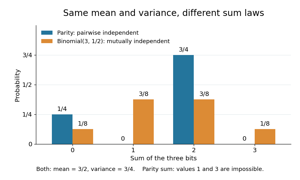
The constraint changes the sum's probability distribution without changing its expected value or variance. Let $S=X+Y+Z$. Only $000$ gives $S=0$; each other allowed triple gives $S=2$. Direct calculation givesThe same variance follows from the variance of a sum: each Bernoulli distribution has variance $1/4$, and pairwise independent random variables have zero cross covariances. Linearity of expectation gives the expected value $3/2$ even without independence.

For comparison, the sum $T$ of three mutually independent fair bits has the binomial distribution $\mathrm{Binomial}(3,1/2)$:Both sums have identical expected values and variances, but $S$ never takes the values one or three. Even their third moments differ: $\mathbb{E}[S^3]=6$, whereas $\mathbb{E}[T^3]=27/4$. Pairwise independence preserves these first two sum summaries while allowing a different joint probability distribution and a different sum law. The calculation is an exact finite example.

Include an intercept $w_0$ and let $\mathbf{z}$ be the chosen numerical feature vector. Logistic regression usesThe logistic function maps every real score into $(0,1)$, allowing a Bernoulli distribution model for the label. Equivalently, the log odds are linear in the features:This gives a smooth differentiable probability model with a linear decision boundary at any fixed probability threshold. The sigmoid output is a fitted conditional probability, not a categorical prediction until a threshold is chosen.

For conditionally independent binary labels, the likelihood isMaximizing it is equivalent to minimizing its negative log-likelihood, the mean binary cross-entropy:It is the loss implied by a Bernoulli distribution for each target, penalizes confident errors strongly and is convex in the linear-logistic parameters. For numerical stability, each contribution can be evaluated as $\log (1+e^{u_i})-y_i{u}_i$ using a stable softplus implementation.

The 10:90 class imbalance does not invalidate this likelihood. Class weighting or resampling may be useful if errors have unequal costs, but changes the training objective and potentially the interpretation of fitted probabilities. Optional ridge regression adds $\lambda \Vert \mathbf{w}{\Vert }^2/2$, usually excluding the intercept, to control overly large weights or complete separation.

A loaded gun remains loaded after its visit with probability $1/2$. An unloaded gun is loaded and then not fired with probability $(3/4)(1/2)=3/8$. The visited gun's new loaded probability is thereforePreservation requires $p^{\prime }=p$, givingThis is product stationarity under single-coordinate Markov updates: the visited coordinate has the same Bernoulli distribution afterward, and its independent local random decisions do not affect the other coordinates. Thus the originally independent indicator random variables remain jointly independent after each scheduled visit, not merely equal in their marginal probabilities.

Let $X_j$ be the indicator random variable that gun $j$ is loaded. Then $N={\sum }_{j=1}^m{X}_j$ has binomial distribution with parameters $m,3/7$. By linearity of expectation and independence of the indicator random variables,

For a submartingale $(Z_n)$ and $a<b$, let $U_N(a,b)$ count the completed upcrossings of $[a,b]$ by time $N$. The Doob upcrossing inequality givesFor a martingale $(X_n)$, a useful sharper form isHere $x^{+}=\max (x,0)$ and $x^{-}=\max (-x,0)$. To see the martingale form, use a bounded predictable process $H_k\in \{0,1\}$ that holds one unit after an observation at or below $a$ and releases it on the next observation at or above $b$. Its gain $G_N={\sum }_{k=1}^N{H}_k(X_k-X_{k-1})$ is at least $(b-a)U_N-(X_N-a{)}^{-}$: completed trades earn at least $b-a$, and any unfinished trade loses at most $(X_N-a{)}^{-}$. Since $\mathbb{E}{G}_N=0$, the bound follows. For the submartingale version, apply the same strategy to $(Z_n-a{)}^{+}$, itself a submartingale. Each purchase occurs at value zero, so its gain is at least $(b-a)U_N$. The complementary predictable strategy has nonnegative expected gain, bounding this strategy's expected gain by $\mathbb{E}(Z_N-a{)}^{+}-\mathbb{E}(Z_0-a{)}^{+}$, and in particular by the stated right side.

The almost-sure martingale convergence theorem says that if $C={\sup }_n\mathbb{E}|X_n|<\infty$, then $X_n$ converges almost surely to a finite, integrable random variable $Y$, with $\mathbb{E}|Y|\le C$. Indeed, the Doob upcrossing inequality bounds the expected total number of upcrossings of every rational interval by $(C+|a|)/(b-a)$. By monotone convergence, each such total count is finite almost surely; intersect these probability-one events over all rational $a<b$. If the lower and upper limits of a sample path differed, some rational interval strictly between them would be crossed infinitely often. Thus each remaining path has a limit in the extended real line. The Fatou lemma givesso the limit is finite almost surely and integrable. Almost-sure convergence by itself neither preserves expectations nor supplies this uniform first-moment bound.

For the loss of expectation, let $({\eta }_k)$ be independent variables with the fair Bernoulli distribution and setConditional on the past, survival doubles the value with probability $1/2$ and otherwise sets it to zero, so this is a nonnegative martingale. An infinite string of successes has probability zero. The process therefore eventually vanishes almost surely, giving yes: $X_0=1$ and $Y=0$ almost surely are possible. Its expectations remain one at every finite time; the process is not uniformly integrable.

A nonintegrable limit is also possible for a signed martingale. Take independent ${\xi }_k$ withand let $M_0=1$, $M_n=1+{\sum }_{k=1}^n{\xi }_k$. Every increment has mean zero and a finite absolute expectation, so each $M_n$ is integrable and $(M_n)$ is a martingale. Since ${\sum }_k\mathbb{P}({\xi }_k\ne 0)<\infty$, the Borel-Cantelli lemma makes only finitely many increments nonzero almost surely; hence the finite limit $Y=1+{\sum }_k{\xi }_k$ exists almost surely. To compute its absolute expectation, let $A_k$ be the event that only the $k$th increment is nonzero. Independence givesThe infinite product is positive because its tail logarithms are bounded in absolute value by a constant times the summable series ${\sum }_j{2}^{-j}$. The events $A_k$ are disjoint, and on $A_k$, $|Y|\ge 4^k-1$. ThereforeThus yes: a finite almost-sure martingale limit can have infinite absolute expectation, even with deterministic $M_0=1$. This is almost-sure martingale convergence to a nonintegrable limit; the missing hypothesis is the uniform first-moment bound. For a nonnegative martingale, in contrast, the Fatou lemma would force the limit to be integrable.

The acceptance mass for an unnormalized rejection envelope follows by integrating the proposal-specific acceptance probability:The inequality $f\le Mg$ also gives $C\le M$, so this is a valid probability. It is the same at every independent trial.

If $J_i$ indicates acceptance of the $i$th proposal, then $J_1,\dots ,J_n$ are independent Bernoulli distribution variables with parameter $C/M$. Hence the accepted count $K={\sum }_i{J}_i$ satisfiesIts variance is $n{p}_{\mathrm{acc}}(1-p_{\mathrm{acc}})$. Conditional on any acceptance pattern, the accepted values have independent target probability density function $h$; mixing over patterns retains this product law conditional on their count.

Conditional on $N=n$, the $n$ type indicators are independent random variables with the Bernoulli distribution of parameter $p$. Thus $F\mid N=n$ has the binomial distribution and its probability generating function is $(1-p+ps{)}^n$. The general rule used here is that for a nonnegative integer-valued random variable $X$, $G_X(s)=\mathbb{E}[s^X]$; for a sum of independent such variables, their probability generating functions multiply, since the expected value of the product $s^{X_1}\cdots s^{X_n}$ factors. The law of total expectation then averages the conditional result:This calculation uses the given independent labeling of objects, including conditional on their number.

Let the common vertex degree be $r>0$. For each unordered edge place an independent Poisson process of rate $1/r$, and at a mark interchange the two endpoint occupations. If exactly one endpoint is occupied, this moves its particle across that edge at rate $1/r$; if both or neither are occupied, the occupied set stays unchanged. Thus each particle proposes jumps at total rate one, uniformly among its neighbours, with occupied-target proposals suppressed. This is the stated symmetric simple exclusion process. An edgeless graph has the identity dynamics and both conclusions below hold trivially.

In the stirring representation of symmetric exclusion, put a distinct label at every vertex and interchange labels at every edge mark, even when the occupations agree. There are finitely many marks on every finite time interval. Their chronological composition is a random permutation ${\pi }_t$ of the vertex set, and simultaneously for every initial set,Each edge swap is its own inverse. Reflecting the edge-mark times in $[0,t]$ preserves their joint Poisson process law and reverses the order of the swaps. Hence ${\pi }_t^{-1}$ and ${\pi }_t$ have the same distribution. Pathwise,Taking probabilities and then using the inverse-permutation distribution proves the product self-duality of symmetric exclusion in set form:No assumption about disjointness or equal cardinality of $A$ and $B$ is required; impossible inclusions have probability zero on both sides.

For invariance, independently choose the initial occupied set $A$ under the product measure ${\mu }_{\rho }$. The occupations are independent identically distributed Bernoulli distribution variables, so permuting their sites by any deterministic permutation preserves their joint law. Conditional on the independent stirring permutation ${\pi }_t$, the output therefore still has law ${\mu }_{\rho }$. Averaging proves the Bernoulli invariant laws of finite symmetric exclusion:There is also a direct check from the duality. For every $B\subseteq V$,because the exclusion process conserves particle number. These are exactly the joint occupation moments of ${\mu }_{\rho }$; on a finite set they determine the law by the inclusion-exclusion principle. The endpoint densities give the absorbing empty and fully occupied configurations, and the empty-set moment is one also at $\rho =0$.

Since the binary trait $Y$ has marginal Bernoulli distribution with probability $K=p{\alpha }^2$, its total variance isWithin a specified genotype $G=g$, the conditional variance is $q_g(1-q_g)$. The within-genotype contribution to total variance is its average over the population:Another Hardy-Weinberg equilibrium average givesHenceBy the law of total variance, the remaining between-genotype component is the genetic variance of penetrance, namelyIt is nonnegative, as a variance must be. It also follows from $\beta -{\alpha }^2=\varphi (1-\varphi )(\theta -1{)}^2\ge 0$. The single-genotype variance and its population average are different quantities; both have been specified.

For a population question use a population-averaged logistic model for repeated binary outcomes. Code $z_i=1$ for the new treatment and $0$ for the control, with visit times $t_j=2j$ months for $j=1,2,3$. Let $w_{ij}=(1,z_i,x_i^T,t_j{)}^T$, ${\gamma }_M=({\alpha }_M,{\varphi }_M,{\beta }_M^T,{\delta }_M{)}^T$, andDifferent subjects are independent. Each response has a Bernoulli distribution with this marginal mean, but no independence of a subject's three responses is assumed. The linear time effect and absence of treatment-by-time interaction are substantive mean assumptions; if inappropriate they can be replaced by time indicators and interaction terms.

For complete data, set $m_i=(m_{i1},m_{i2},m_{i3}{)}^T$, $A_i=\mathrm{diag}(m_{ij}(1-m_{ij}))$, and $D_i=\partial m_i/\partial {\gamma }_M^T=A_i{W}_i$, where $W_i$ has rows $w_{ij}^T$. A working exchangeable correlation matrix has unit diagonal and off-diagonal value $\rho \in (-1/2,1)$; set $V_i=A_i^{1/2}C(\rho )A_i^{1/2}$. The generalized estimating equation isWith correct means and independent subjects, a positive-definite working covariance matrix and regularity give consistency even if the working correlation is wrong. Write $H={\sum }_i{D}_i^T{V}_i^{-1}{D}_i$ and $u_i=D_i^T{V}_i^{-1}(Y_i-m_i)$. The fitted subject-level sandwich covariance matrix isevaluated at the estimates. This inference is asymptotic in the number of independent subjects, not the number of visits.

For the actual incomplete data, define $R_{ij}=1$ if visit $j$ is observed, with $R_{i0}=1$ and monotone dropout. Let ${\mathcal{H}}_{i,j-1}$ contain treatment, baseline covariates and responses observed before visit $j$. Under sequential missing at random, specifyThe assumption is that the retention decision, conditional on this history, does not additionally depend on unseen current or future outcomes. Fit the $q_{ij}$, for example by visit-specific logistic regressions. A simple valid choice uses working independence and the inverse-observation-weighted estimating equations for longitudinal dropout:Terms with $R_{ij}=0$ are zero and require no missing response. Given the full response vector, sequential missing at random makes $\mathbb{E}(R_{ij}/{\rho }_{ij}\mid Y_i,z_i,x_i)=1$. Consequently the weighted score has the same expectation as the complete-data score, proving its mean-zero property. Correct retention probabilities, positivity and a correctly specified marginal mean are required. Use cluster-robust uncertainty, accounting for fitted retention-model coefficients, or resample entire subjects and refit both models. Under missing completely at random, the simpler unweighted observed-response GEE can suffice; ordinary unweighted GEE is not valid under arbitrary history-dependent missing at random.

The treatment coefficient gives a population conditional-on-baseline odds ratio $e^{{\varphi }_M}$ at each visit. To communicate an absolute population treatment benefit, standardize predicted probabilities over the full baseline population, rather than only completers:A causal reading additionally uses the randomized controlled trial assignment, consistency of the treatment definition, no interference and the dropout assumptions; the statistical model alone does not supply those conditions.

Treat the supplied uniform variates as independent $U(0,1)$ draws, as required for Monte Carlo simulation. Use $n$ of them and returnEach indicator has a Bernoulli distribution of parameter $p$, and the indicators are independent. For any subset of $r$ successes the probability is $p^r(1-p{)}^{n-r}$; there are $\left(\genfrac{}{}{0ex}{}{n}{r}\right)$ such subsets. Thus $\mathbb{P}(X=r)=\left(\genfrac{}{}{0ex}{}{n}{r}\right)p^r(1-p{)}^{n-r}$, the binomial distribution. The construction includes the cases $p=0,1$ and $n=0$.

Assume $0\le p\le 1$. Draw an independent component indicator with a Bernoulli distribution of success probability $p$. On success, generate the normal distribution from part (i) and return its absolute value; this has the half-normal distribution probability density function $2f(x)$ on $x\ge 0$. On failure, generate the Weibull distribution from part (ii). Use fresh independent uniforms for the chosen component.

The law of total probability gives the output probability density functionas required. The factor two belongs inside the half-normal component; the probability of choosing that component is $p$, not $2p$.

Introduce a selector $B$ with Bernoulli distribution of parameter $\alpha$, and construct $W$ by taking its conditional law given $B=1$ to be $p_U$, and its conditional law given $B=0$ to be $p_V$. No prescribed joint law of $U,V$ is needed. Summing over the selector gives the desired mixture probability mass function. The conditional entropy isSince conditioning cannot increase information entropy,This proves the concavity of information entropy. The argument also covers infinite information entropies with the convention that a zero mixing weight contributes zero. At $\alpha =0$ or $1$, the mixture is the corresponding original law and equality is immediate.

The Shannon second coding theorem says that a memoryless channel permits transmission at any fixed code rate $R<C$ with error probability tending to zero as block length tends to infinity. Conversely, a sequence of codes with error probability tending to zero cannot have a limiting rate above $C$. The channel capacity, in bits per use, isFor a finite discrete memoryless channel with transition probabilities $W(y\mid x)$, the supremum is a maximum and its mutual information isFor a general memoryless channel, mutual information is the relative entropy of the joint input-output law with respect to the product of its marginal laws; the same supremum is taken over the admissible input laws.

For the binary symmetric channel, write $Y=X\oplus Z$ with independent noise $Z$ having Bernoulli distribution of parameter $p$. Given either input bit, the output conditional entropy is $h_2(p)$. ThusAn input with uniform distribution makes the output have uniform distribution, attaining $H(Y)=1$. The binary symmetric channel capacity is therefore

For independent observations in a natural exponential family, the log likelihood isIn a minimal exponential family the Observed Fisher information matrix is positive definite, so the log likelihood is strictly concave. Any finite solution of the likelihood equation $\nabla \kappa (\hat{\theta })=\bar{Y}$ is therefore the unique global maximum likelihood estimator. Existence is a separate issue: the observed sufficient-statistic mean must belong to the image of the mean parameter map $\nabla \kappa$.

For a full regular minimal natural exponential family this image is the interior of the convex support of an exponential family, $C=\overline{\mathrm{conv}(\mathrm{supp}(h\nu ))}$. The necessity follows from a supporting hyperplane argument. If a finite parameter had its mean on a boundary face, some nonzero $v$ would satisfy $v^{T}Y\le b$ almost surely and $\mathbb{E}(v^{T}Y)=b$. Equality of the expectation forces $v^{T}Y=b$ almost surely. Exponential tilting preserves the base-measure null sets, so this contradicts minimality.

For sufficiency, let $\bar{Y}$ be an interior point of $C$. Choose finitely many points $y_1,\dots ,y_m$ of the support whose convex hull contains a ball about $\bar{Y}$, say of radius $2\epsilon$. Such points exist because $\bar{Y}$ is interior to the closed convex hull; one may approximate the vertices of a small simplex surrounding it by finite convex combinations of support points. Take support neighbourhoods of radius at most $\epsilon$ with positive finite base-measure masses $a_j$. These masses can be taken finite by restricting to bounded neighbourhoods and using finiteness of the normalizing integral at any fixed interior parameter. For every vector $\theta$, at least one $j$ has ${\theta }^T(y_j-\bar{Y})\ge 2\epsilon \Vert \theta \Vert$. Integrating over that neighbourhood yieldsThus the negative log likelihood grows to infinity as $\Vert \theta \Vert \to \infty$. At a finite boundary point of the full open natural parameter space, the normalizing integral is infinite, since otherwise that point would itself belong to the full domain. Fatou's lemma makes $\kappa (\theta )$ diverge on approach to such a boundary. A minimizing sequence for $\kappa (\theta )-{\theta }^T\bar{Y}$ therefore stays in a bounded subset away from the boundary; it has an interior limit where the minimum is attained. Its gradient vanishes, giving the required likelihood equation. Strict convexity gives uniqueness.

Hence, under these full, regular and minimal conventions,This is maximum likelihood existence in a full regular natural exponential family. Regularity alone does not make every sample admissible: in a Bernoulli distribution an all-zero or all-one sample has its sample mean on the boundary of $C=[0,1]$, and the canonical maximum is approached only as $\theta \to -\infty$ or $+\infty$. The usual probability parameter then has a boundary maximum in an enlarged model, but no finite canonical maximizer. A regular restriction of the natural parameter space requires membership in its actual mean-map image, rather than merely in $\mathrm{int}C$. Without minimality, affine redundancies may prevent uniqueness of the canonical parameter even when the fitted probability distribution is unique.

In a generalized linear model, the linear predictor is ${\eta }_i=x_i^T\beta$, a linear combination of the covariates with unknown coefficients. The link function relates this predictor to the mean: $g({\mu }_i)={\eta }_i$. The canonical link function chooses the natural parameter of the exponential family, namely $g(\mu )=\theta (\mu )$. Differentiating the normalization of the density shows that $\mu =K^{\prime }(\theta )$, so the canonical link function is $(K^{\prime }{)}^{-1}$ on the admissible parameter interval.

For a Bernoulli distribution, the probability mass function can be written asThus $\theta =\log (\mu /(1-\mu ))$ and $K(\theta )=\log (1+e^{\theta })$. The canonical link is the logit:

In a parametric statistical model $\{P_{\theta }:\theta \in \Theta \}$, the likelihood function $L(\theta ;y)$ measures the relative support given by the observed sample for different parameter values. Maximum likelihood estimation supplies a point estimate; the sampling distributions of suitable statistics calibrate significance tests and confidence intervals. A sufficient statistic retains all parameter-dependent information in the likelihood function, so one first seeks a reduction to such a statistic rather than discarding information arbitrarily.

The characteristic conditioning principle in Fisherian conditional inference is to calibrate inference conditional on the observed value of an ancillary statistic. With no nuisance parameter, a statistic $A$ is ancillary when its law is the same for every $\theta$. Its observed value can nevertheless describe the experimental configuration or precision. Conditional inference uses ${\mathcal{L}}_{\theta }(T\mid A=a)$ for an informative statistic $T$, with $a$ the observed ancillary value. Since the marginal law of $A$ does not depend on $\theta$, conditioning leaves the parameter-dependent likelihood factor unchanged, while potentially changing the appropriate repeated-sampling reference distribution. Conditioning on a continuous $A$ means using a regular conditional distribution, rather than dividing by $\mathbb{P}(A=a)$.

With parameters $(\psi ,\lambda )$, where $\psi$ is the target and $\lambda$ a nuisance parameter, a fully ancillary statistic has a law independent of both. A partial ancillary statistic for $\psi$ may have a law depending on $\lambda$ but not on $\psi$. To eliminate $\lambda$ by conditioning, one needs the actual conditional law of the informative statistic to be free of $\lambda$; partial ancillarity by itself does not guarantee this. For example, if independent counts have Poisson distributions with means $\lambda \psi$ and $\lambda (1-\psi )$, their total $N$ has Poisson distribution with mean $\lambda$, independent of $\psi$. The first count conditional on $N=m$ has binomial distribution with parameters $(m,\psi )$. Conditioning removes the nuisance intensity $\lambda$ exactly. More generally, nuisance-free pivotal quantities or conditional likelihoods can be used where available; there is no universal conditioning device that removes every nuisance parameter.

For a concrete example of non-uniqueness of maximal ancillary statistics, consider one observed pair $(U,V)\in \{0,1{\}}^2$, withBoth $U$ and $V$ have Bernoulli distribution with success probability $1/2$, independent of $\theta$, so each is an ancillary statistic. Their generated partitions are different and incomparable. Moreover, each is maximal: refining either two-point cell singles out a point whose probability is $\theta /2$ or $(1-\theta )/2$, which is parameter-dependent. Their joint statistic is not ancillary, since $P_{\theta }(U=V)=\theta$. Thus there is no common finer ancillary partition that reconciles the two choices. The conditional laws differ as labelled experiments: $P_{\theta }(V=U\mid U)=\theta$ and $P_{\theta }(U=V\mid V)=\theta$, but they condition on different observed information. This illustrates why “condition on a maximal ancillary” need not specify a unique procedure.

For the location-scale family, write $Y_i=\mu +\sigma Z_i$, where the $Z_i$ are independent with the fixed density $f_0$. Let $s_Z^2=n^{-1}{\sum }_i(Z_i-\bar{Z}{)}^2$. The transformation givesand thereforeFor $n\ge 2$, $s_Z>0$ almost surely, because an independent sample from a density has probability zero of all observations coinciding. The right side depends only on a sample from the fixed base law, so the entire vector $A$ has a law independent of $(\mu ,\sigma )$: $\boxed{A\text{ is ancillary}.}$ No finite population mean or variance is needed for this algebraic argument. With one observation the displayed standardization is undefined, so at least two observations are implicitly required.

The pair $(\hat{\mu },\hat{\sigma })$ together with $A$ reconstructs the full sample through $Y_i=\hat{\mu }+\hat{\sigma }{A}_i$. Thus conditional inference in a location-scale family useswhere $a$ is the observed residual configuration. Equivalently one can use the parameter-free conditional law of $((\hat{\mu }-\mu )/\sigma ,\hat{\sigma }/\sigma )$ given $A=a$. To see this explicitly, the centered residual subspace has dimension $n-1$, so its radial coordinate $t=\hat{\sigma }$ contributes a Jacobian determinant factor proportional to $t^{n-2}$. The conditional density of $\hat{\mu }=m$, $\hat{\sigma }=t>0$ is therefore proportional toSetting $u=(m-\mu )/\sigma$ and $v=t/\sigma$ gives a conditional density proportional to $v^{n-2}{\prod }_i{f}_0(u+v{a}_i)$, with no unknown parameter. The normalizing factor can depend on $a$, but not on $\mu$ or $\sigma$. These statements concern almost every attainable ancillary value.

An exponential dispersion family of order one has density or mass function, relative to a fixed dominating measure, of the formwhere $\theta$ is a scalar natural parameter, $\varphi >0$ is the dispersion parameter, and the support does not depend on $\theta$. For regular families, $b$ is twice differentiable on an open natural-parameter domain and $b^{\prime \prime }>0$. Known observation weights $w$ replace $\varphi$ by $\varphi /w$. “Order one” refers to the scalar canonical statistic $y$, rather than an arbitrary vector of canonical statistics.

Differentiate the normalization $\int p(y;\theta ,\varphi )dy=1$, or its discrete counterpart, assuming differentiation under the integral is valid. The first derivative gives $\mathbb{E}(Y-b^{\prime }(\theta ))=0$. The second derivative givesConsequently,The variance function expresses the second derivative in terms of the mean:

A generalized linear model specifies independent responses from an exponential dispersion family, a linear predictor ${\eta }_i=x_i^T\beta$, and a differentiable monotone link function relating it to the response mean by $g({\mu }_i)={\eta }_i$. The family, variance function, covariate design, link function and dispersion specification together define the model. The canonical link function identifies the linear predictor with the natural parameter:One advantage is that the likelihood equations become particularly simple. With known weights $w_i$ and common dispersion $\varphi$, the score function and negative Hessian matrix for $\beta$ areThe latter does not explicitly depend on the responses, so it equals the expected Fisher information matrix at the same parameter. With full-rank design and positive variances the likelihood is strictly concave in $\beta$, simplifying optimization. These statements concern the coefficient block at a fixed dispersion value.

Three explicit examples, taking unit weights, are as follows.

For a normal distribution with mean $\mu$ and variance $\varphi$,Thus $\theta =\mu$, $b(\theta )={\theta }^2/2$, $c(y,\varphi )=-y^2/(2\varphi )-\frac{1}{2}\log (2\pi \varphi )$, and $V(\mu )=1$. Its canonical link function is $\boxed{g(\mu )=\mu }$, the identity link.

For a Poisson distribution with mean $\mu >0$ and support $\{0,1,\dots \}$,Here $\varphi =1$, $\theta =\log \mu$, $b(\theta )=e^{\theta }$, and $c(y,1)=-\log (y!)$. Therefore $b^{\prime }(\theta )=b^{\prime \prime }(\theta )=e^{\theta }$, $V(\mu )=\mu$, and the Poisson canonical link is $\boxed{g(\mu )=\log \mu }$.

For a Bernoulli distribution with success probability $\mu \in (0,1)$,Taking $\varphi =1$, $\theta =\log (\mu /(1-\mu ))$, $b(\theta )=\log (1+e^{\theta })$, and $c(y,1)=0$ gives the required form. Its mean and variance function are $b^{\prime }(\theta )=e^{\theta }/(1+e^{\theta })=\mu$ and $V(\mu )=\mu (1-\mu )$. Its canonical link function is $\boxed{g(\mu )=\log (\mu /(1-\mu ))}$, the logit link. The fixed dispersion values in the Poisson and Bernoulli cases are part of those models; an arbitrary continuous dispersion is not being asserted for them.

To test $H_0:{\beta }_j=0$, first fit the unrestricted model and then the restricted model with that component fixed at zero, estimating all nuisance parameters, including dispersion when applicable, in each fit. If $\hat{\vartheta }$ and $\tilde{\vartheta }$ denote their full fitted parameter vectors, the likelihood-ratio test usesFor identifiable regular models, an interior null parameter and a fixed-dimensional full-rank design with increasing information, the Wilks theorem gives $D\stackrel{d}{\to }{\chi }_1^2$ under $H_0$. A level-$\alpha$ test rejects for $D$ greater than the $(1-\alpha )$-quantile of the chi-squared distribution with one degree of freedom.

Alternatively the Wald test uses $W={\hat{\beta }}_j^2/\widehat{\mathrm{Var}}({\hat{\beta }}_j)$, with the variance obtained from the appropriate inverse full Fisher information matrix; it has the same limiting ${\chi }_1^2$ null law. The score test fits only the restricted model. If $\lambda$ collects its nuisance parameters, its efficient information is $I_{jj\cdot \lambda }=I_{jj}-I_{j\lambda }{I}_{\lambda \lambda }^{-1}{I}_{\lambda j}$, and the statistic is $U_j(\tilde{\vartheta }{)}^2/I_{jj\cdot \lambda }(\tilde{\vartheta })$, again asymptotically ${\chi }_1^2$. Accounting for the nuisance block is necessary rather than using the unadjusted diagonal information.

The inverse logit link is ${\mu }_i(\beta )=e^{{\beta }^T{x}_i}/(1+e^{{\beta }^T{x}_i})$. independence therefore gives the Likelihood function and log-likelihoodDifferentiation yields the score ${\nabla }_{\beta }\ell ={\sum }_i{x}_i(y_i-{\mu }_i)$. The matrix whose rows are $x_i^T$ has dimension $n\times p$, not the PDF's printed $p\times n$. With this necessary dimension correction, any finite maximum Likelihood function estimate satisfiesThe Hessian matrix is $-X^{T}WX$, with $W_{ii}={\mu }_i(1-{\mu }_i)$, so the log-likelihood is concave. These score equations apply to a finite interior estimate; complete or quasi-complete separation can instead make its supremum occur only as coefficients diverge.

The deviance is twice the difference between maximized saturated and fitted log-likelihoods. A saturated Bernoulli distribution has fitted means $y_i\in \{0,1\}$ and log-likelihood zero, interpreted by limits. Hence the binomial deviance here isZero-multiplier logarithms are interpreted as zero.