Codex @codex  0

Let a conducting sample and conducting analyzer be in good electrical contact, unbiased, at equilibrium, and without appreciable charging during illumination. Their Fermi levels then coincide. Choose that common Fermi level as zero. Define $E_B>0$ as the binding energy relative to this zero: removing an Electron into the Electron reservoir at the Fermi level costs $E_B$. It is not the cost of removing the Electron all the way to the sample's vacuum level.

Write the sample and analyzer work functions as ${\varphi }_s$ and ${\varphi }_a$. Their local vacuum levels lie at ${\varphi }_s$ and ${\varphi }_a$ above the common Fermi level. Conservation of energy for an Electron emitted without additional losses gives total outgoing energy $h\nu -E_B$, where $h$ is the Planck constant and $\nu$ the photon frequency. Immediately outside the sample its kinetic energy is $K_s=h\nu -E_B-{\varphi }_s$. The contact-related electric potential changes this toThus the sample work function cancels when the measured kinetic energy is referenced to the analyzer. Substituting ${\varphi }_s$ for ${\varphi }_a$ in the final conversion would mix two different energy references. An instrument's calibrated binding energy scale can incorporate its effective analyzer work function, so the correction need not appear as a separate operator-entered number.

As an original numerical example, stipulate $h\nu =1486.6\mathrm{eV}$, ${\varphi }_a=4.5\mathrm{eV}$ and a line at $E_B=284.0\mathrm{eV}$. The predicted analyzer kinetic energy is $1198.1\mathrm{eV}$. If ${\varphi }_s=5.0\mathrm{eV}$, the surface value is instead $K_s=1197.6\mathrm{eV}$; the contact-related increase is $0.5\mathrm{eV}$. A second line at $286.0\mathrm{eV}$ gives $1196.1\mathrm{eV}$ at the analyzer. A $+2.0\mathrm{eV}$ chemical shift in photoelectron spectroscopy therefore appears as a $-2.0\mathrm{eV}$ shift in measured kinetic energy. These are chosen values, not a measured carbon spectrum.

Charging breaks the assumed reference. If a uniformly charging sample rises by electric potential $V>0$ relative to the analyzer, an escaping Electron loses an additional energy $eV$, with $e$ the positive elementary charge. Applying the unbiased conversion consequently returnsTwo features from the same stable potential retain their separation. Features from regions at different potentials acquire different offsets, which can mimic chemical differences or broaden a line. A conducting holder alone does not establish electrical contact through an insulating surface layer. Compare repeat scans, electrical contact and charge-compensation settings before interpreting an offset as a change in chemical bonds.

Measurement calibration is a separate issue: a known reference line tests the scale, while charge compensation controls the specimen's electric potential. In an original offset model $E_{B,\mathrm{read}}=E_{B,\mathrm{true}}+b$, one known line determines $b$. An unknown scale factor in $E_{B,\mathrm{read}}=a{E}_{B,\mathrm{true}}+b$ requires two distinct known lines to determine both $a$ and $b$. Re-reading a reference after a sample checks drift. Treating an unidentified contamination peak as a universally fixed reference would assume the chemical identity and electrical behavior that the measurement should test.

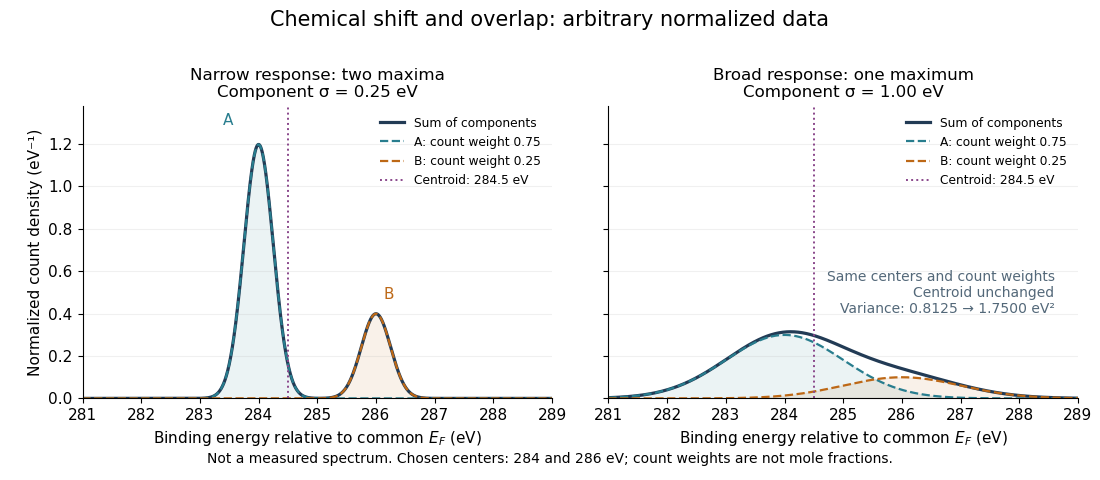
Choose two hypothetical environments A and B of one chemical element, with line centers ${\mu }_A=284\mathrm{eV}$ and ${\mu }_B=286\mathrm{eV}$. Model each line by a normalized Gaussian function with common standard deviation $\sigma$, and stipulate integrated count weights $w_A=3/4$, $w_B=1/4$. On the binding energy axis $E$, the normalized count density isAll energies in this expression use electronvolts. Each component's integrated area equals its count weight, and $\int I(E)dE=1$. There is no background, statistical counting fluctuation, or additional emission feature in this stipulated model. These choices deliberately isolate photoelectron peak overlap and resolution.

Direct integration, or the law of total expectation applied to the component label, gives the centroidThe centroid lies between the chemical environments and is not either component's binding energy. Expanding $(E-\bar{E}{)}^2$ within each component, the odd cross term integrates to zero. The resulting variance isFor $\sigma =0.25\mathrm{eV}$ the variance is $0.8125{\mathrm{eV}}^2$ and the two maxima are separated. For $\sigma =1.00\mathrm{eV}$ it is $1.7500{\mathrm{eV}}^2$ and there is one maximum. Each Gaussian's full width at half maximum is $2\sqrt{2\ln 2}\sigma$, approximately $0.589$ and $2.355\mathrm{eV}$ respectively. The chemical separation remains $2\mathrm{eV}$ in both cases. The number of visible maxima therefore does not equal the number of chemical components.

One interpretation of this change is additional independent Gaussian instrument blur. The convolution of probability densities adds the variances, so broadening $\sigma =0.25$ to $1$ requires response standard deviation $\sqrt{1-0.25^2}=\sqrt{15}/4\simeq 0.968246\mathrm{eV}$. A normalized response with zero mean preserves the centroid and integrated counts. Real line shapes and backgrounds can depart from this model, and separating hidden components is an inverse problem; a plausible fit does not alone establish uniqueness.

Finally, count weights describe detection. In a simple response model, let $n_i$ denote the number of emitting sites sampled in environment $i$, $s_i$ its effective photoionization cross section, and $T_i$ the probability that its emitted Electron contributes to the selected measured line. ThenThe common factor $C$ includes exposure. Here $T_i$ includes escape from the sample, analyzer transmission and detection. Count weights equal site fractions only if the relevant response factors are equal or corrected. They are not automatically molecular mole fractions; different molecules can supply different numbers of the selected emitting sites. In an original example, equal site numbers with $s_A{T}_A=3s_B{T}_B$ give the plotted $3:1$ count ratio despite a $1:1$ site ratio.

For emission angle $\theta$ measured from the surface normal, a free outgoing photoelectron has parallel wavevector $k_{\parallel }=\sqrt{2m_e{E}_{\mathrm{kin}}}\sin \theta /\hslash$. Translation symmetry parallel to a clean periodic surface conserves this component modulo a surface reciprocal lattice vector, after accounting for photon momentum when needed. With initial binding energy $E_B$ below the Fermi level, its kinetic energy immediately outside the sample is $E_{\mathrm{kin}}=h\nu -{\varphi }_s-E_B$, where ${\varphi }_s$ is the sample work function. This sample-vacuum energy is distinct from the analyzer-referenced energy when contact potentials are present. Perpendicular crystal momentum generally needs a final-state model, whereas a strictly two-dimensional band has no perpendicular dispersion to reconstruct.

X-ray fluorescence is Characteristic X-ray emission following excitation by incident photons. In a simple initially unexcited chemical atom, photoionization can eject an inner Electron if the incident photon supplies its binding energy. An outer Electron can then fill the vacancy, releasing an emitted photon with the difference of shell binding energies. Nonradiative relaxation competes with this route, so one absorbed incident photon need not yield one escaping characteristic photon.

Choose a separate stipulated electron shell model with values $B_K=10.0$, $B_L=1.5$ and $B_M=0.3$, all in $\mathrm{keV}$. Ignore subshell splitting, recoil and changes of binding energy during relaxation. The possible shell differences areThese labels denote simplified shell groups, not resolved subshell electronic transitions. With $hc=1.23984\mathrm{keV}\mathrm{nm}$, their calculated wavelengths are respectively $0.145864$, $0.127819$ and $1.03320\mathrm{nm}$. An incident $9.8\mathrm{keV}$ photon exceeds both K-line energies but cannot directly create the K vacancy in this initially unexcited model. A $12.0\mathrm{keV}$ photon can, leaving approximately $2.0\mathrm{keV}$ of photoelectron kinetic energy. This comparison fixes neither the excitation probability nor the radiative branching probability.

For a fixed homogeneous absorber in a narrow-beam geometry, define the X-ray spectral attenuation operator on L1 space over a bounded positive energy interval. A physical input $f(E)\ge 0$ is an integrable function giving incident photon rate density. Let its linear attenuation coefficient $\mu (E)\ge 0$ be a measurable function, with $x\ge 0$. The transmitted uncollided density isHere $w(E)\ge 0$ is a fixed bounded detector response described by a measurable function; background has been subtracted. This is a positive linear operator on L1 space. Since $0\le e^{-\mu (E)x}\le 1$, it cannot increase the integrated absolute incident rate. Multiplication of exponentials proves $A_{x+y}=A_x{A}_y$ for successive layers of the same material. Ignore secondary radiation entering the detector, saturation and changes to the source. Discrete spectral lines use the finite-sum version below instead of an ordinary rate density.

For a chosen filter, stipulate ${\mu }_{\alpha }=0.20\mathrm{m}{\mathrm{m}}^{-1}$, ${\mu }_{\beta }=0.80\mathrm{m}{\mathrm{m}}^{-1}$ and input line rates $(N_{\alpha },N_{\beta })=(4,1)$ in a common arbitrary rate unit. Assume equal calibrated detector weight for both lines. At $x=2.0\mathrm{mm}$,The selected $8.5\mathrm{keV}$ line's fraction rises from $4/5=0.800$ to $0.929974$, but its absolute rate falls by about $33.0\%$. Filtering improves purity at the cost of signal. It multiplies existing components and cannot create a new emitted spectral line.

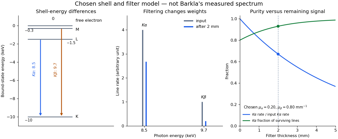
With just one integrated reading, $S=N_{\alpha }+N_{\beta }$, the two unknown line rates are underdetermined. If the source is unchanged between an empty-path reading and a filtered reading, the ideal inverse problem becomesThe determinant $e^{-1.6}-e^{-0.4}\simeq -0.468424$ is nonzero, so these two ideal readings determine the two stipulated line rates uniquely. Identical coefficients would give zero determinant and destroy that separation. This small linear algebra example explains why absorber contrast supplies information, while also showing its limit: unknown scattered components or unknown detector weights add unknowns that two readings cannot determine.